A hospital administrator wants to study the association between patient satisfaction and patients age, severity of illness and anxiety level. 23 patients were randomly selected and the data were collected, where larger values of satisfaction, severity, and anxiety are associated with more satisfaction, increased severity of illness and more anxiety, respectively.
d <-read.table("data/patsat.txt", header =TRUE)head(d)
  Satisfaction        Age           Severity        Anxiety
 Min.   :26.00   Min.   :28.00   Min.   :43.00   Min.   :1.800
 1st Qu.:50.00   1st Qu.:33.00   1st Qu.:48.00   1st Qu.:2.150
 Median :60.00   Median :40.00   Median :50.00   Median :2.300
 Mean   :61.35   Mean   :39.61   Mean   :50.78   Mean   :2.296
 3rd Qu.:73.50   3rd Qu.:44.50   3rd Qu.:53.50   3rd Qu.:2.400
 Max.   :89.00   Max.   :55.00   Max.   :62.00   Max.   :2.900
10.2 Relationships between pairs of variables
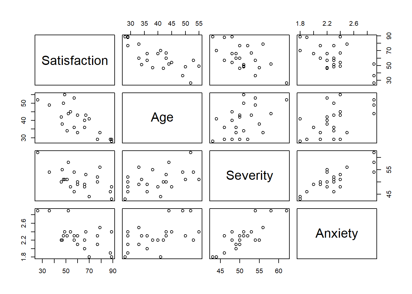
We summarise the data graphically using a matrix of scatterplots to examine all pairwise relationships.
All explanatory variables by themselves are negatively and linearly related to Satisfaction.
The variable Age shows the strongest relationship with Satisfaction, followed by Anxiety and then Severity.
We need to perform a formal analysis using multiple regression to see which combination of variables is most useful to predict Satisfaction.
10.3 Collinearity
Collinearity occurs when two or more explanatory variables in a multiple regression model are highly correlated.
If the explanatory variables are strongly related to each other then it is possible that they may affect the response in the same way and this makes it difficult to distinguish their contributions.
If this is the case, then it is likely that we would not need to use all the explanatory variables in the model. That is, we have some redundant explanatory variables.
Collinearity causes instability in the estimation of \(\boldsymbol{\beta}\) but it is not so much of a problem for prediction.
We will try to avoid having very similar predictors in the model.
10.4 Regression equation
res <-lm(Satisfaction ~ Age + Severity + Anxiety, data = d)summary(res)
Call:
lm(formula = Satisfaction ~ Age + Severity + Anxiety, data = d)

Residuals:
    Min      1Q  Median      3Q     Max
-16.954  -7.154   1.550   6.599  14.888

Coefficients:
            Estimate Std. Error t value Pr(>|t|)
(Intercept) 162.8759    25.7757   6.319 4.59e-06 ***
Age          -1.2103     0.3015  -4.015  0.00074 ***
Severity     -0.6659     0.8210  -0.811  0.42736
Anxiety      -8.6130    12.2413  -0.704  0.49021
---
Signif. codes:  0 '***' 0.001 '**' 0.01 '*' 0.05 '.' 0.1 ' ' 1

Residual standard error: 10.29 on 19 degrees of freedom
Multiple R-squared:  0.6727,    Adjusted R-squared:  0.621
F-statistic: 13.01 on 3 and 19 DF,  p-value: 7.482e-05
mean patient satisfaction decreases by 1.210 for every unit increase in age holding the rest of variables constant
mean patient satisfaction decreases by 0.666 for every unit increase in severity of illness holding the rest of variables constant
mean patient satisfaction decreases by 8.6 for every unit increase in anxiety holding the rest of variables constant
10.5 Tests for coefficients. t test
Test null hypothesis ‘response variable \(Y\) is not linearly related to variable \(X_i\)’ versus alternative hypothesis ‘\(Y\) is linearly related to \(X_i\)’, \(i=1,\ldots,p\)
Distribution: t(n-p-1) where \(p\) is the number of \(\beta\) parameters excluding \(\beta_0\)
t distribution with degrees of freedom = number of observations - number of explanatory variables - 1
p-value: probability of obtaining a test statistic as least as extreme as the observed assuming the null is true
\(H_1: \beta_i \neq 0\) is \(P(T\geq |t|)\)
summary(res)
Call:
lm(formula = Satisfaction ~ Age + Severity + Anxiety, data = d)

Residuals:
    Min      1Q  Median      3Q     Max
-16.954  -7.154   1.550   6.599  14.888

Coefficients:
            Estimate Std. Error t value Pr(>|t|)
(Intercept) 162.8759    25.7757   6.319 4.59e-06 ***
Age          -1.2103     0.3015  -4.015  0.00074 ***
Severity     -0.6659     0.8210  -0.811  0.42736
Anxiety      -8.6130    12.2413  -0.704  0.49021
---
Signif. codes:  0 '***' 0.001 '**' 0.01 '*' 0.05 '.' 0.1 ' ' 1

Residual standard error: 10.29 on 19 degrees of freedom
Multiple R-squared:  0.6727,    Adjusted R-squared:  0.621
F-statistic: 13.01 on 3 and 19 DF,  p-value: 7.482e-05
p-value=0.001 hence there is strong evidence that age affects the mean patient satisfaction allowing for severity and anxiety.
p-value=0.421 hence there is not evidence that severity affects the mean patient satisfaction allowing for age and anxiety.
p-value=0.490 hence there is not evidence that anxiety affects the mean patient satisfaction allowing for age and severity.
10.6 Confidence interval for the slope \(\beta_i\)
A \((1-\alpha)\times 100\)% confidence interval for the slope \(\beta_1\) is \[\hat \beta_i \pm t^* \times SE_{\hat \beta_i}\]
\(t^*\) is the value on the \(t(n-p-1)\) density curve with area \(c\) between the critical points \(-t^*\) and \(t^*\). That is, \(t^*\) is the value such that \(\alpha/2\) of the probability in the \(t(n-p-1)\) distribution is below \(t^*\).
10.7 ANOVA Table
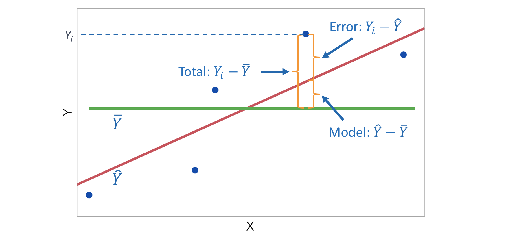
The total variation in the response \(Y\) is partitioned between two sources: variation due to the model and variation due the residuals.
Sources of variation are:
Model (or Regression)
Error (or Residual)
Total
Sum of Squares
\[SSM + SSE = SST\]
\[SSM = \sum_{i=1}^n (\hat Y_i - \bar Y)^2\]
\[SSE = \sum_{i=1}^n (Y_i - \hat Y_i)^2\]
\[SST = \sum_{i=1}^n (Y_i - \bar Y)^2\]Degrees of Freedom
Test null hypothesis ‘none of the explanatory variables are useful predictors of the response variable’ versus alternative hypothesis ‘at least one of the explanatory variables is related to the response variable’
\(H_0\): \(\beta_{1} =\beta_{2}=...=\beta_{p}\) = 0 (all coefficients are 0)
\(H_1\): at least one of \(\beta_1\), \(\beta_2\), \(\dots\), \(\beta_p \neq\) 0 (not all coefficients are 0)
ANOVA table for multiple regression
Source
Sum of Squares
degrees of freedom
Mean square
F
p-value
Model
SSM
p
MSM=SSM/p
MSM/MSE
Tail area above F
Error
SSE
n-p-1
MSE=SSE/(n-p-1)
Total
SST
n-1
The total variation in the response \(Y\) is partitioned between two sources: variation due to the model, i.e., because \(Y\) changes as the \(X\)’s change, and variation due the residuals, i.e., the scatter above and below the fitted regression surface.
\[F = \frac{\sum_{i=1}^n (\hat Y_i - \bar Y)^2/p}{\sum_{i=1}^n (Y_i - \hat Y_i)^2/(n-p-1)} = \frac{SSM/df_M}{SSE/df_E} = \frac{MSM}{MSE},\] where \(p\) is the number of \(\beta\) parameters excluding \(\beta_0\) in \(Y= \beta_0 + \beta_1 X_1 + \beta_2 X_2 + \ldots + \beta_p X_p + \epsilon\).
Under \(H_0\), distribution of \(F \sim F(p, n-p-1)\)
\(F\) has an F distribution with degrees of freedom = (number of explanatory variables, number of observations - number of explanatory variables - 1)
p-value: probability that test statistic has a value as extreme or more extreme than the observed
p-value = \(P(F \geq F_{\mbox{observed}})\)
If p-value < \(\alpha\) (or F larger than the critical value), we reject the null hypothesis.
There is evidence that at least one of the regression coefficients \(\beta_i, i=1,\ldots,p\) is non-zero. Thus, at least one of the explanatory variables \(X, i=1,\ldots,p\) is useful for predicting \(Y\) (we don’t know which one though). There is evidence that at least one (one or more) of the explanatory variables in the model is potentially useful for predicting the response in the linear model.
If p-value > \(\alpha\) (or F smaller than the critical value), we fail to reject the null hypothesis.
There is no evidence that any of the explanatory variables can help model the response variable using this kind of model. We cannot conclude that any of the explanatory variables is useful for prediction \(Y\).
summary(res)
Call:
lm(formula = Satisfaction ~ Age + Severity + Anxiety, data = d)

Residuals:
    Min      1Q  Median      3Q     Max
-16.954  -7.154   1.550   6.599  14.888

Coefficients:
            Estimate Std. Error t value Pr(>|t|)
(Intercept) 162.8759    25.7757   6.319 4.59e-06 ***
Age          -1.2103     0.3015  -4.015  0.00074 ***
Severity     -0.6659     0.8210  -0.811  0.42736
Anxiety      -8.6130    12.2413  -0.704  0.49021
---
Signif. codes:  0 '***' 0.001 '**' 0.01 '*' 0.05 '.' 0.1 ' ' 1

Residual standard error: 10.29 on 19 degrees of freedom
Multiple R-squared:  0.6727,    Adjusted R-squared:  0.621
F-statistic: 13.01 on 3 and 19 DF,  p-value: 7.482e-05
p-value=0.000 \(< \alpha = 0.05\). There is strong evidence that at least one of the explanatory variables in the model is related to the response.
Root Mean Square Error (RMSE)
\[RMSE = \sqrt{\sum_{i=1}^n (Y_i - \hat Y_i)^2/(n-p-1)} = \sqrt{MSE}\] RMSE is ‘Residual standard error: 10.29 on 19 degrees of freedom’ in output
10.9 R\(^2\)
R\(^2\) (R-squared or coefficient of determination) is the proportion of variation of the response variable \(Y\) (vertical scatter from the regression surface) that is explained by the model (explained by the changes in the \(x\)’s).
\[R^2 = \frac{\mbox{variability explained by the model}}{\mbox{total variability}} = 1 - \frac{\mbox{variability in residuals}}{\mbox{total variability}}\]
R\(^2\) measures how successfully the regression explains the response.
If the data lie exactly on the regression surface then R\(^2\) = 1.
If the data are randomly scattered then R\(^2\) = 0.
For simple linear regression, R\(^2\) is equal to the square of the correlation between \(Y\) and \(X\), \(R^2 = r^2\)
\[R^2 = \frac{SSM}{SST} = \frac{\sum_{i=1}^n (\hat Y_i - \bar Y)^2}{\sum_{i=1}^n ( Y_i - \bar Y)^2} \ \ \ \mbox{(proportion of variability explained by the model)}\] or equivalently
\[R^2 = 1 - \frac{SSE}{SST} = 1 - \frac{\sum_{i=1}^n ( Y_i - \hat Y_i)^2}{\sum_{i=1}^n ( Y_i - \bar Y)^2} \ \ \ \mbox{(1 - proportion of variability not explained by the model)}\]
10.10 R\(^2\)(adj)
\(R^2\) will increase as more explanatory variables are added to a regression model. However, adding more explanatory variables does not necessarily lead to a better model. We look at R\(^2\)(adj).
R\(^2\)(adj) or Adjusted R-squared is the proportion of variation of the response variable explained by the fitted model adjusting for the number of parameters.
We use the adjusted \(R^2\) to assess goodness of fit of the model when comparing models with different numbers of parameters.
\[R^2(adj) = 1 - \frac{SSE/(n-p-1)}{SST/(n-1)} = 1 - \frac{SSE}{SST} \times \frac{n-1}{n-p-1},\] where \(n\) is the number of observations and \(p\) is the number of predictor variables in the model. Because \(p\) is never negative, \(R^2(adj)\) will be smaller than the unadjusted \(R^2\).
In this example, R\(^2\)(adj)= 62.10% The percentage of variation explained by the model is about 62% adjusting for the number of parameters.