21 Exponential family
21.1 Generalized linear models (GLMs)
Generalized linear models allow for response distributions other than normal, and for a degree of non-linearity in the model structure.
A GLM is defined by specifying two components:
- The response should be a member of the exponential family distribution.
- The link function describes how the mean of the response and a linear combination of the predictors are related.
Specifically, a GLM makes the distributional assumptions that the \(Y_i\) are independent and
\(Y_i \sim\) some exponential family distributions (e.g., normal, Poisson, Binomial, Gamma).
\[g(\mu_i) = \boldsymbol{X}_i' \boldsymbol{\beta}\]
- \(\mu_i = E(Y_i)\)
- \(g\) is a smooth monotonic link function
- \(\boldsymbol{\beta}\) is a vector of unknown parameters
- \(\boldsymbol{X}_i'=(X_{1i}, \ldots, X_{pi})\) is the \(i\)th row of a model matrix \(\boldsymbol{X}\).
Because GLMs are specified in terms of the linear predictor \(\boldsymbol{\eta} \equiv \boldsymbol{X \beta}\), many of the general ideas and concepts of linear modeling carry over, to generalized linear modeling.
21.2 Exponential family of distributions
In a GLM the distribution of the response variable \(Y_i\) comes from a distribution in the exponential family with probability density function
\[f(y_i;\theta_i,\phi)=\exp\left\{{y_i\theta_i -b(\theta_i)\over a_i(\phi)}+c(y_i,\phi)\right\}.\]
Here \(\theta_i\) is an unknown parameter that is a function of the mean, \(\phi\) is a dispersion parameter that may or may not be known, and \(a_i(\phi)\), \(b(\theta_i)\) and \(c(y_i, \phi)\) are known functions.
- \(\theta_i\) is called canonical parameter and represents the location
- \(\phi\) is called dispersion parameter and represents the scale
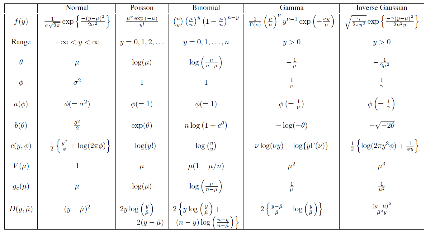
The exponential family includes as special cases many common distributions. Some exponential family distributions:
Note: In Binomial distribution, \(\mu = n \pi\)
Normal or Gaussian
\[f(y) = \frac{1}{\sqrt{2\pi}\sigma} exp\left(-\frac{(y-\mu)^2}{2 \sigma^2}\right)= exp\left( \frac{y \mu-\mu^2/2}{\sigma^2} - \frac{1}{2}\left( \frac{y^2}{\sigma^2} + log(2 \pi \sigma^2) \right) \right)\]
So we can write
- \(\theta = \mu\)
- \(\phi = \sigma^2\)
- \(a(\phi)= \phi\)
- \(b(\theta) = \theta^2/2\)
- \(c(y, \phi) = -(y^2/\phi+ log(2\pi \phi))/2\)
Poisson
\[f(y) = e^{-\mu}\mu^y/y! = exp(y \log(\mu)-\mu-\log(y!))\] So we can write
- \(\theta = \log(\mu)\)
- \(\phi = 1\)
- \(a(\phi)= 1\)
- \(b(\theta) = exp(\theta)\)
- \(c(y, \phi) = -\log(y!)\)
Binomial
\[f(y) ={n \choose y} \pi^y (1-\pi)^{n-y} =\] \[exp \left( y \log \pi + (n-y) \log(1-\pi) + \log {n \choose y} \right) = exp \left( y \log \frac{\pi}{1-\pi} + n \log{(1-\pi)} + \log {n \choose y} \right)\]
So we can write
- \(\theta = \log \frac{\pi}{1-\pi}\) (then \(\pi = \frac{e^\theta}{1+e^\theta}\) so \(1-\pi = \frac{1}{1+e^\theta}\))
- \(b(\theta) = - n \log(1-\pi) = n \log(1+ exp(\theta))\)
- \(c(y, \phi) = \log{n \choose y}\)
- \(\phi = 1\)
- \(a(\phi)= 1\)
21.2.1 Mean and variance of the exponential family distributions
If \(Y_i\) has a distribution in the exponential family then it has mean and variance
\[E(Y_i) = b'(\theta_i)\] \[Var(Y_i) = b''(\theta_i) a_i(\phi),\]
where \(b'(\theta_i)\) and \(b''(\theta_i)\) are the first and second derivatives of \(b(\theta_i)\).
That is, the mean is a function of the location only, while the variance is a product of functions of the location and the scale.
Normal
- \(\theta = \mu\)
- \(\phi = \sigma^2\)
- \(a(\phi)= \phi\)
- \(b(\theta) = \theta^2/2\)
\[E(Y) = b'(\theta) = (\theta^2/2)' = \theta = \mu\] \[Var(Y) = b''(\theta) a(\phi) = (\theta)' a(\phi) = a(\phi) = \sigma^2\]
Poisson
- \(\theta = \log(\mu)\)
- \(\phi = 1\)
- \(a(\phi)= 1\)
- \(b(\theta) = exp(\theta)\)
\[E(Y) = b'(\theta) = (exp(\theta))' = exp(\theta) = \mu\]
\[Var(Y) = b''(\theta) a(\phi) = (exp(\theta))' a(\phi) = exp(\theta) = \mu\]
Binomial
- \(\theta = \log \frac{\pi}{1-\pi}\) (then \(\pi = \frac{e^\theta}{1+e^\theta}\) so \(1-\pi = \frac{1}{1+e^\theta}\))
- \(b(\theta) = - n \log(1-\pi) = n \log(1+ exp(\theta))\)
- \(\phi = 1\)
- \(a(\phi)= 1\)
\[E(Y) = b'(\theta) = ( n \log(1+ exp(\theta)))' = n \frac{exp(\theta)}{1+exp(\theta)} = n \pi = \mu\] Differentiating again using the quotient rule \(\left( (g/h)' = (g'h-gh')/h^2 \right)\)
\[Var(Y) = b''(\theta) a(\phi) = \left(n \frac{e^\theta}{1+e^\theta }\right)' = n \frac{e^{\theta}}{(1+e^{\theta})^2} = n \frac{e^{\theta}}{(1+e^{\theta})} \frac{1}{(1+e^{\theta})} = n \pi(1-\pi) = \mu (1 - \mu/n)\]
Derivation mean and variance of the exponential family distributions
\[E(Y) = b'(\theta)\] \[Var(Y) = b''(\theta) a(\phi)\]
The log-likelihood for a single \(y\) is given by
\[l(\theta) = (y \theta - b(\theta))/a(\phi) + c(y, \phi)\] Taking derivatives with respect to \(\theta\) gives
\[l'(\theta) = (y - b'(\theta))/a(\phi)\]
Taking expectation over \(y\) gives
\[E[l'(\theta)] = (E[Y]-b'(\theta))/a(\phi)\] From likelihood theory, we know \(E[l'(\theta)]=0\) at the true value of \(\theta\) so
\[E[Y]=\mu=b'(\theta)\]
Taking second derivatives:
\[l''(\theta) = - b''(\theta)/a(\phi)\]
From likelihood theory, we know \(E[l''(\theta)]=-E[(l'(\theta))^2]\). We evaluate at the true value of \(\theta\) and obtain
\[b''(\theta)/a(\phi) = E[(Y-b'(\theta))^2]/a^2(\phi)\] (\(l''(\theta) = - b''(\theta)/a(\phi)\) and \(E[l''(\theta)] = - b''(\theta)/a(\phi)\))
(\(l'(\theta) = (y - b'(\theta))/a(\phi)\) and \(E[l'(\theta)^2] = E[(y - b'(\theta))^2/a(\phi)^2]\))
which gives
\[Var[Y]= E[(Y-b'(\theta))^2] = b''(\theta) a(\phi)\]
21.2.2 Variance function
\[E(Y) = b'(\theta)\] \[Var(Y) = b''(\theta) a(\phi),\]
\(a(\phi)\) could in principle be any function of \(\phi\), and when working with GLMs there is no difficulty in handling any form of \(a(\phi)\), if \(\phi\) is known. However, when \(\phi\) is unknown matters become awkward, unless we can write \(a(\phi) = \phi/w\), where \(w\) are known weights that may vary between observations. For example, \(a(\phi) = \phi/w\) allows the possibility of unequal variances in models based on the normal distribution, but in most cases \(w\) is simply 1.
Then we have
\[Var(Y) = b''(\theta) \frac{\phi}{w}\]
Subsequently it is convenient to write \(Var(Y)\) as a function of \(\mu = E(Y)\)
\[Var(Y)=V(\mu)\phi\]
\[V(\mu) = \frac{b''(\theta)}{w} = \frac{b''(b'^{-1}(\mu))}{w}\]
The variance function \(V(\mu)\) describes how the variance relates to the mean (\(Var(Y)=V(\mu)\phi\)) using the known relationship between \(\theta\) and \(\mu\), \(E[Y] = \mu = b'(\theta)\), \(b'^{-1}(\mu) = \theta\).
Example: In the normal case, \(b(\theta)= \theta^2/2\) and \(b''(\theta)=1\) and so the variance is independent of the mean \(Var(Y)=V(\mu)\phi = 1 \times \sigma^2\).
21.3 The link function
The second element of the generalization is that instead of modeling the mean, we introduce a one-to-one continuous differentiable transformation \(g(\mu_i)\) and focus on
\[\eta_i = g(\mu_i)\]
\(g(\cdot)\) is called link function. Examples include the identity, log and logit.
We assume that the transformed mean follows a linear model \[\eta_i = \beta_0 + \beta_1 x_{i1} + \ldots + \beta_p x_{ip} = \boldsymbol{x_i' \beta}\] \(\eta_i\) is called linear predictor.
Since the link function is one-to-one we can invert it to obtain \[\mu_i = g^{-1}(\boldsymbol{x_i' \beta})\]
Note that we do not transform the response \(y_i\) but rather its expected value \(\mu_i\). A model where \(\log(y_i)\) is linear on \(x_i\), for example, is not the same as a generalized linear model where \(\log(\mu_i)\) is linear on \(x_i\).
Example: The standard linear model can be described as a GLM with normal errors and identity link so that \(\eta_i = \mu_i\). It also happens that \(\mu_i\) is equal to the \(\theta_i\), the parameter in the exponential family density.
Canonical link
We say that we have a canonical link when the link function makes the linear predictor \(\eta_i\) the same as the canonical parameter \(\theta_i\).
- The identity is the canonical link for the normal distribution.
- The logit is the canonical link for the binomial distribution
- The log is the canonical link for the Poisson distribution.