20 Count, binary and normal data

Learning objectives

Generalized linear models (GLMs)
Binary data
Count data
Normal data

21 The general linear model

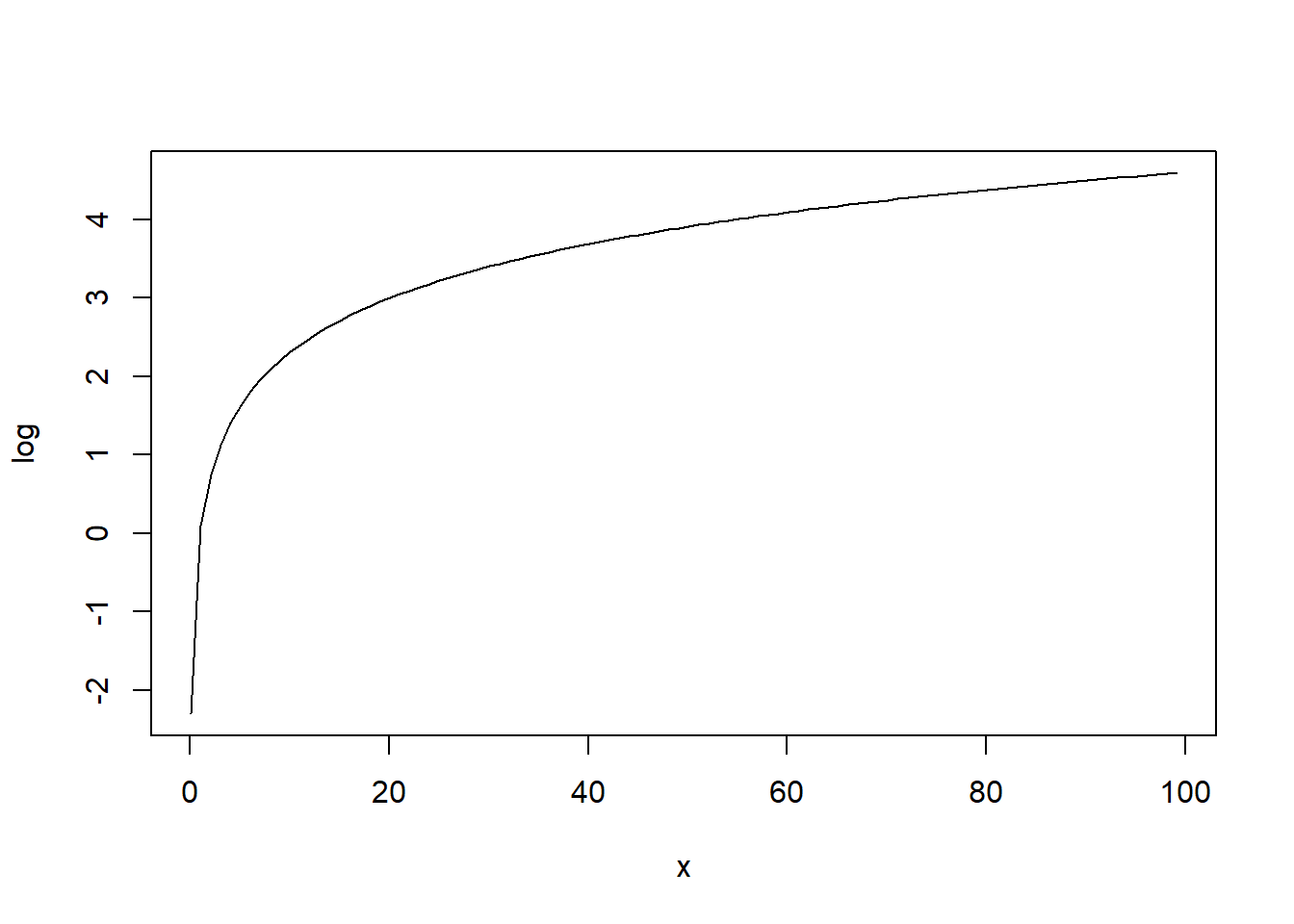
In a general linear model, the response \(Y_i\), \(i = 1, \ldots, n\), is modeled as a linear function of explanatory variables \(x_i\), \(j=1, \ldots, p\) plus an error term:

\[Y_i = \beta_0 + \beta_1 x_{1i} + \ldots + \beta_p x_{pi} + \epsilon_i,\]

where we assume errors \(\epsilon_i\) are independent and identically Gaussian distributed with \(E[\epsilon_i] = 0,\ \ Var[\epsilon_i] = \sigma^2\).

Here general refers to the dependence on potentially more than one explanatory variable, versus the simple linear model:

\[Y_i = \beta_0 + \beta_1 x_{i} + \epsilon_i\]

The model is linear in the parameters, e.g.,

\[Y_i = \beta_0 + \beta_1 x_1 + \beta_2 x_1^2 + \epsilon_i\]

but not, e.g.,

\[Y_i = \beta_0 + \beta_1 x_1^{\beta_2} + \epsilon_i\]

Although a very useful framework, there are some situations where general linear models are not appropriate.

In a general linear model the response variable is a continuous variable (e.g., BMI, systolic blood pressure). We can have other situations when the response variable is binary or a count.

Generalized linear models (GLMs) extend the general linear model framework to address these issues.

22 Generalized linear models (GLMs)

A generalized linear model (GLM) makes the distributional assumptions that the \(Y_i\) are independent and

\(Y_i \sim\) distribution from exponential family (e.g., normal, Poisson, Binomial).

The link function describes how the mean of the response and a linear combination of the predictors are related

\[\eta_i = g(\mu_i) = \beta_0 + \beta_1 x_{1i} + \ldots + \beta_p x_{pi}\]

The link function describes how the mean of the response, \(E[Y_i]=\mu_i\) depends on the linear predictor: \(g(\mu_i) = \eta_i\)
The variance function describes how the variance depends on the mean \(Var(Y_i) = V(\mu)\phi\), where the dispersion parameter \(\phi\) is a constant

Here we will see how to model the following data:

Poisson data
Binomial data
Gaussian data

23 Modeling Poisson data

Count data, in which there is no upper limit to the number of counts, may represent counts or rates which are counts per unit of time/area/distance, etc.

For example,

number of household burglaries in a city in a given year
number of customers served by a saleperson in a given month
number of train accidents in a given year

In such situations, the counts can be assumed to follow a Poisson distribution

\[Y_i \sim Po(\mu_i)\] Then \[E(Y_i)=\mu_i\] \[Var(Y_i)=\mu_i\]

Link function must map from \((0, \infty)\) to \((-\infty, \infty)\). A natural choice is \[\eta_i = g(\mu_i)=\log(\mu_i)\]

x <- seq(0.1, 100, 1)
plot(x, log(x), type = "l", xlab = "x", ylab = "log")

The inverse of the log function is the exponential function: exp(log(mu)) = mu

The inverse of the log function maps real values to \((0, \infty)\).

x <- seq(-2, 5, 0.1)
plot(x, exp(x), type = "l", xlab = "log", ylab = "x")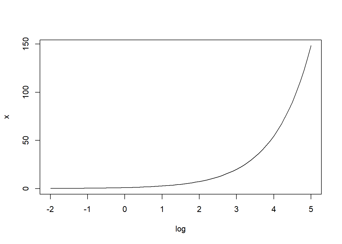

Poisson GLM with the log link is known as log-linear model.

Canonical link function for Poisson data is the log link.

\[\log(\mu) = \beta_0 + \beta_1 x_1 + \ldots + \beta_j x_j + \ldots + \beta_p x_p\]

If we increase \(x_j\) by one unit

\[\log(\mu^*) = \beta_0 + \beta_1 x_1 + \ldots + \beta_j (x_j+1) + \ldots + \beta_p x_p\] \[\log(\mu^*) - \log(\mu) = \beta_j\]

\[\log\left(\frac{\mu^*}{\mu}\right) = \beta_j\]

\[\frac{\mu^*}{\mu}= exp(\beta_j)\]

\[\mu^* = exp(\beta_j) \mu\]

\(exp(\beta_j)\) is called relative risk (risk relative to some baseline)

Therefore,

\(\beta_j\) is the increase or decrease in the log of the mean associated with one-unit increase in \(x_j\), holding all other variables constant

\[\log\left(\mu\ \ |_{x_j+1}\right)-\log\left(\mu\ \ |_{x_j}\right) = \beta_j\]

\(exp(\beta_j)\) \[\frac{\mu\ |_{x_j+1}} {\mu \ |_{x_j}} = exp(\beta_j)\]
When \(x_j\) increases one unit, the mean is multiplied by \(exp(\beta_j)\)

\[\mu |_{x_j+1} = \mu |_{x_j} \times exp(\beta_j)\]

23.1 Example Poisson (counts)

Consider an experiment designed to evaluate the effectiveness of an anti-fungal chemical on plants. A total of 60 plant leaves infected with a fungus were randomly assigned to treatment with 0, 5, 10, 15, 20, or 25 units of the anti-fungal chemical, with 10 plant leaves for each amount of anti-fungal chemical. Following a two-week period, the leaves were studied under a microscope, and the number of infected cells was counted and recorded for each leaf.

d <- read.csv("data/glms-LeafInfectionData.txt")
head(d)

Plot observed number of infected cells for each amount of anti-fungal treatment.

plot(d$x, d$y, xlab = "Amount of anti-fungal treatment", ylab = "Number of infected cells")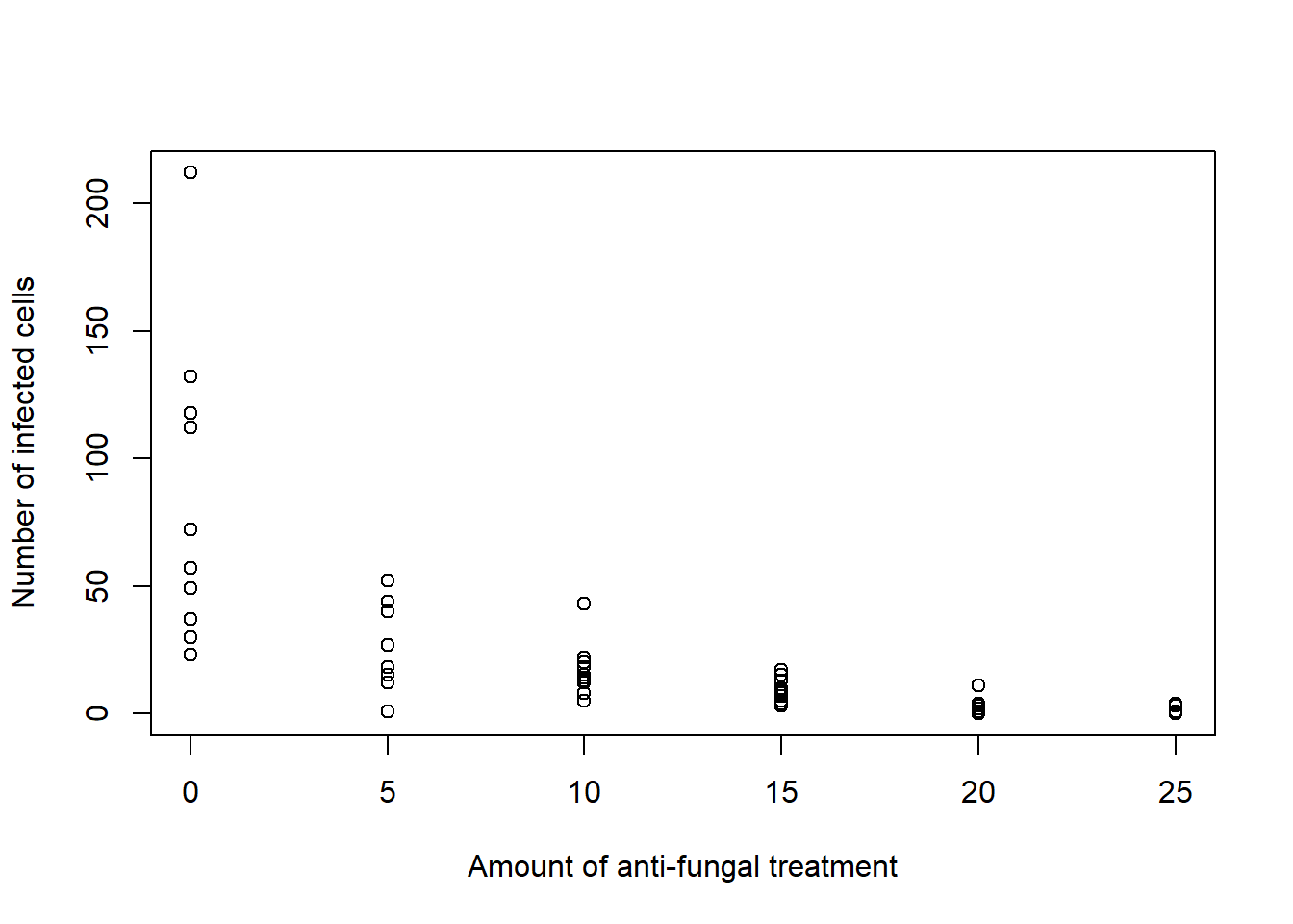

res <- glm(y ~ x, family = "poisson", data  = d)
summary(res)


Call:
glm(formula = y ~ x, family = "poisson", data = d)

Coefficients:
             Estimate Std. Error z value Pr(>|z|)    
(Intercept)  4.373003   0.032434  134.83   <2e-16 ***
x           -0.162011   0.004933  -32.84   <2e-16 ***
---
Signif. codes:  0 '***' 0.001 '**' 0.01 '*' 0.05 '.' 0.1 ' ' 1

(Dispersion parameter for poisson family taken to be 1)

    Null deviance: 2314.87  on 59  degrees of freedom
Residual deviance:  614.65  on 58  degrees of freedom
AIC: 849.53

Number of Fisher Scoring iterations: 5

\[\log(\mu) = 4.37 -0.16 \times x\]

For one unit increase in the amount of anti-fungal chemical, the log of the mean number of infected cells decreases by 0.16.

When the amount of anti-fungal chemical increases by one unit, the mean number of infected cells is multiplied by exp(-0.162011) = 0.85.

Predictions

Now we predict the mean number of infected cells per leaf as a function of the amount of anti-fungal chemical.

We have \(\log(\mu) = \beta_0 + \beta_1 x\). That is, \(\mu = exp(\beta_0 + \beta_1 x)\).

Then, the mean number of infected cells for a leaf treated with \(x\) units of the anti-fungal chemical can be estimated by \(exp(\hat \beta_0 + \hat \beta_1 x)\).

# Predict at these chemical amounts
xamount <- seq(0, 25, by = 0.1)
# Coefficients
b <- coef(res)
# Predictions
predictions <- exp(b[1] + b[2]*xamount)
# Plot
plot(d$x, d$y, xlab = "Amount of anti-fungal treatment", ylab = "Number of infected cells")
lines(xamount, predictions, col = "red")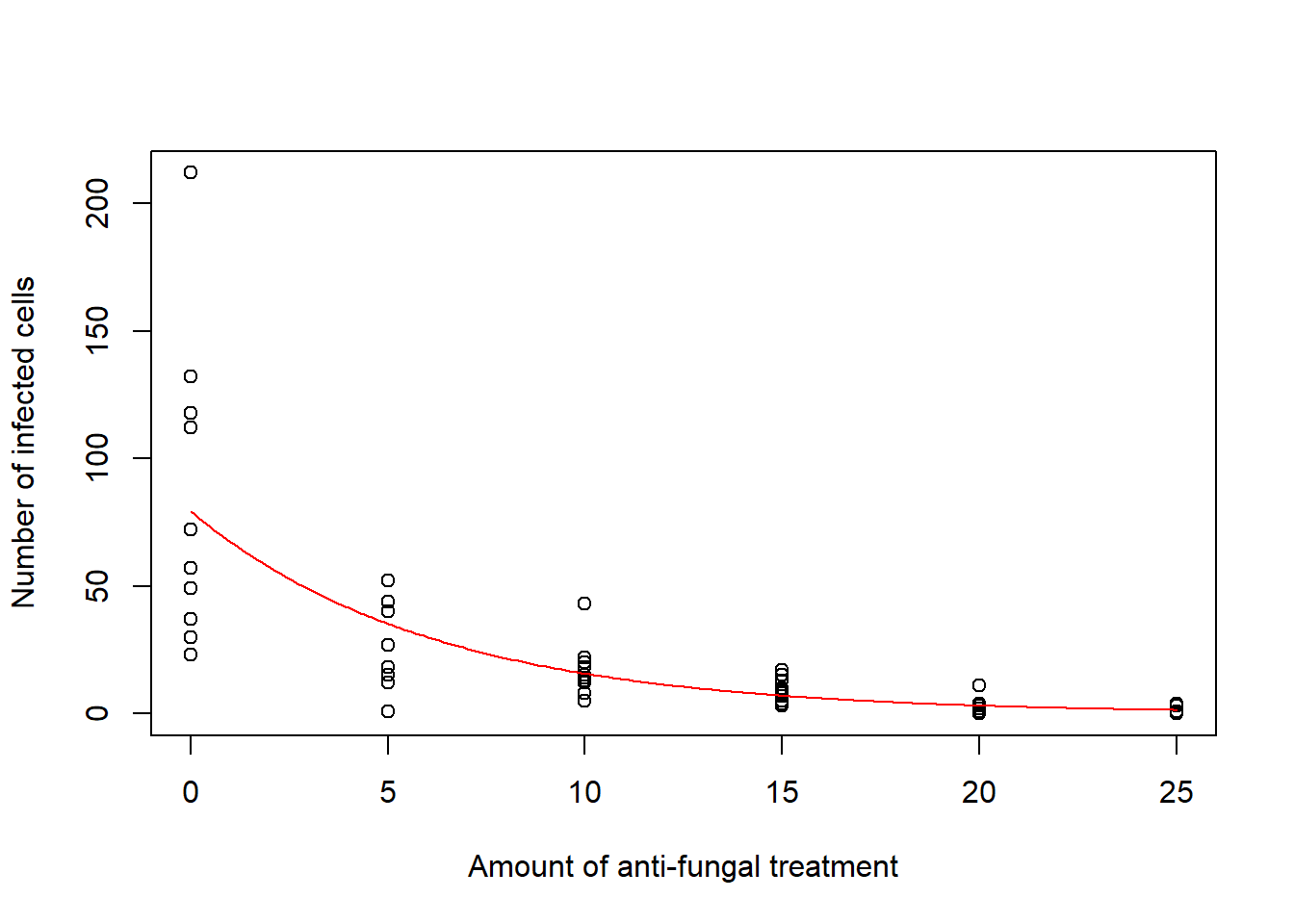

We can also use the function predict(object, newdata, type, ...) to obtain predictions (?predict.glm):

object is the glm fitted object
newdata is a data frame with the variables with which to predict. If omitted, the fitted linear predictors are used.
type is type of prediction. When type = "link" predictions are on the scale of the linear predictors (log in the case of Poisson data, log-odds in the case of Binomial data). When type = "response" predictions are on the scale of the response variable (mean in the case of Poisson data, probabilities in the case of Binomial data).

Type "response" (mean)

# Predict at these chemical amounts
xamount <- seq(0, 25, by = 0.1)
# Predictions
predictions <- predict(res, data.frame(x = xamount), type = "response")
# Plot
plot(d$x, d$y, xlab = "Amount of anti-fungal treatment", ylab = "Number of infected cells")
lines(xamount, predictions, col = "red")

Type "link" (log(mean))

# Predict at these chemical amounts
xamount <- seq(0, 25, by = 0.1)
# Predictions
predictions <- predict(res, data.frame(x = xamount), type = "link")
# Plot
plot(xamount, predictions, col = "red", type = "l",
xlab = "Amount of anti-fungal treatment", ylab = "log(number of infected cells)")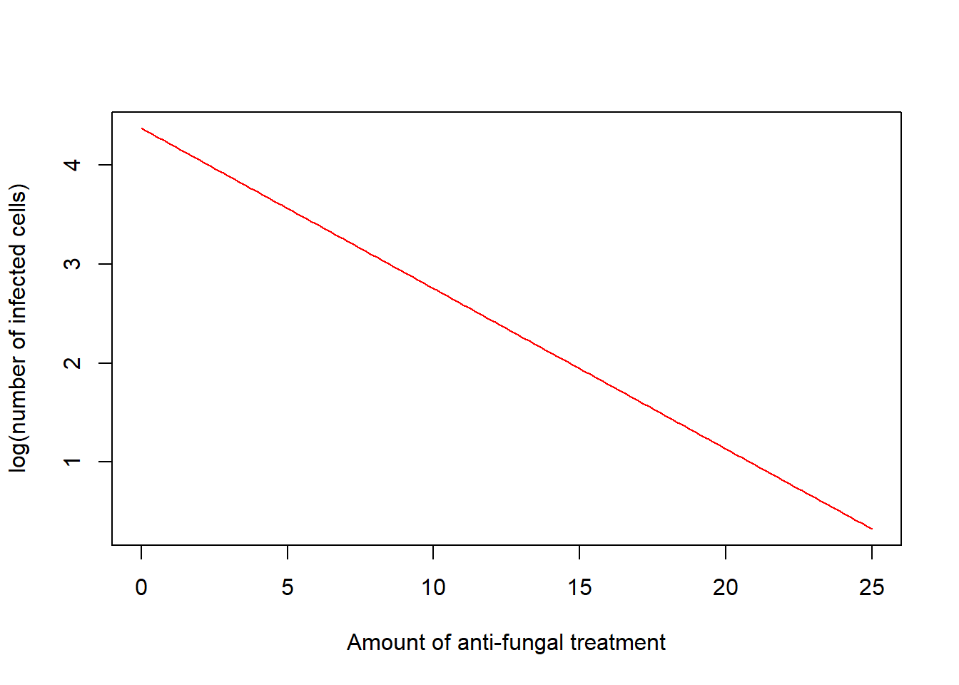

23.2 Exercise Poisson (counts)

Some female crabs attract many males while others do not attract any. The males that cluster around a female are called satellites. In order to understand what influences the presence of satellite crabs, researchers selected female crabs and collected data on the following characteristics:

number of male satellites
width of her carapace shell (in centimeters)
condition of her spine (bad, good, middle)
color of her shell (dark, darker, light, medium)
weight of the female (in grams)

Interpret coefficients of the following model:

library("glmbb")
data("crabs")
# In the data, variable y denotes as.numeric(satell > 0)
dim(crabs)

[1] 173   6

head(crabs)

   color spine width satell weight y
1 medium   bad  28.3      8   3050 1
2   dark   bad  22.5      0   1550 0
3  light  good  26.0      9   2300 1
4   dark   bad  24.8      0   2100 0
5   dark   bad  26.0      4   2600 1
6 medium   bad  23.8      0   2100 0

summary(crabs)

    color       spine         width          satell           weight    
 dark  :44   bad   :121   Min.   :21.0   Min.   : 0.000   Min.   :1200  
 darker:22   good  : 37   1st Qu.:24.9   1st Qu.: 0.000   1st Qu.:2000  
 light :12   middle: 15   Median :26.1   Median : 2.000   Median :2350  
 medium:95                Mean   :26.3   Mean   : 2.919   Mean   :2437  
                          3rd Qu.:27.7   3rd Qu.: 5.000   3rd Qu.:2850  
                          Max.   :33.5   Max.   :15.000   Max.   :5200  
       y         
 Min.   :0.0000  
 1st Qu.:0.0000  
 Median :1.0000  
 Mean   :0.6416  
 3rd Qu.:1.0000  
 Max.   :1.0000

res <- glm(satell ~ width + spine, family = "poisson", data = crabs)
summary(res)


Call:
glm(formula = satell ~ width + spine, family = "poisson", data = crabs)

Coefficients:
            Estimate Std. Error z value Pr(>|z|)    
(Intercept) -3.12469    0.56497  -5.531 3.19e-08 ***
width        0.15668    0.02096   7.476 7.69e-14 ***
spinegood    0.09899    0.10490   0.944    0.345    
spinemiddle -0.10033    0.19309  -0.520    0.603    
---
Signif. codes:  0 '***' 0.001 '**' 0.01 '*' 0.05 '.' 0.1 ' ' 1

(Dispersion parameter for poisson family taken to be 1)

    Null deviance: 632.79  on 172  degrees of freedom
Residual deviance: 566.60  on 169  degrees of freedom
AIC: 929.9

Number of Fisher Scoring iterations: 6

23.3 Modeling rates

In many cases we are making comparisons across observation units \(i = 1, \ldots, n\) with different levels of exposure to the event and hence the measure of interest is the rate of occurrence. For example,

number of household burglaries per 10,000 households in city \(i\) in a given year
number of customers served per hour by salesperson \(i\) in a given month
number of train accidents per billion train-kilometers in year \(i\)

Since the counts are Poisson distributed, we would like to use a GLM to model the expected rate, \(\lambda_i=\mu_i/t_i\), where \(t_i\) is the exposure for unit \(i\).

Typically explanatory variables have a multiplicative effect rather than an additive effect on the expected rate, therefore a suitable model is

\[Y_i \sim Po(\mu_i)\]

\[\mu_i = \lambda_i t_i\]

\[\log(\mu_i/t_i)= \log(\lambda_i) = \beta_0 + \beta_1 x_{1i} + \ldots + \beta_p x_{ip}\]

\[\log(\mu_i)= \log(t_i) + \log(\lambda_i) = \log(t_i) + \beta_0 + \beta_1 x_{1i} + \ldots + \beta_p x_{ip}\]

\(\log(t_i)\) is an offset: a term with a fixed coefficient of 1.

Offsets are easily specified to glm(), either using the offset argument (offset = log(time)) or using the offset function in the formula (+ offset(log(time))).

Examples of offsets. When modeling the number of disease cases in regions, the offset is the population of each region. When modeling the number of accidents in periods of time, the offset is the length of the period of time for each observation.

If all the observations have the same exposure, the model does not need an offset term and we can model \(\log(\mu_i)\) directly.

\(\beta_j\) is the increase or decrease in the log of the expected rate associated with one-unit increase in \(x_j\), holding all other variables constant

\[\log\left(\lambda\ \ |_{x_j+1}\right)-\log\left(\lambda\ \ |_{x_j}\right) = \beta_j\]

\(exp(\beta_j)\) \[\frac{\lambda\ |_{x_j+1}} {\lambda \ |_{x_j}} = exp(\beta_j)\]
When \(x_j\) increases one unit, the expected rate is multiplied by \(exp(\beta_j)\)

\[\lambda |_{x_j+1} = \lambda |_{x_j} \times exp(\beta_j)\]

23.4 Example Poisson (rates)

The ships data from the MASS package contains the number of ships damage incidents caused by waves and aggregate months of service by ship type, year of construction, and period of operation. The variables are

incidents number of damage incidents
service aggregate months of service
type type: A to E
year year of construction: 1960-64, 65-69, 70-74, 75-79
period period of operation: 1960-74, 75-79

Here it makes sense to model the expected number of incidents per aggregate months of service. Let us consider a log-linear model including all the variables.

library(MASS)


Attaching package: 'MASS'

The following object is masked _by_ '.GlobalEnv':

    crabs

data(ships)
# We exclude ships with 0 months of service
ships2 <- subset(ships, service > 0)
# Convert period and year to factor variables
ships2$year <- as.factor(ships2$year)
ships2$period <- as.factor(ships2$period)
summary(ships2)

 type  year    period     service        incidents    
 A:7   60: 9   60:15   Min.   :   45   Min.   : 0.00  
 B:7   65:10   75:19   1st Qu.:  371   1st Qu.: 1.00  
 C:7   70:10           Median : 1095   Median : 4.00  
 D:7   75: 5           Mean   : 4811   Mean   :10.47  
 E:6                   3rd Qu.: 2223   3rd Qu.:11.75  
                       Max.   :44882   Max.   :58.00

res <- glm(incidents ~ type + year + period, family = "poisson", data = ships2, offset = log(service))
summary(res)


Call:
glm(formula = incidents ~ type + year + period, family = "poisson", 
    data = ships2, offset = log(service))

Coefficients:
            Estimate Std. Error z value Pr(>|z|)    
(Intercept) -6.40590    0.21744 -29.460  < 2e-16 ***
typeB       -0.54334    0.17759  -3.060  0.00222 ** 
typeC       -0.68740    0.32904  -2.089  0.03670 *  
typeD       -0.07596    0.29058  -0.261  0.79377    
typeE        0.32558    0.23588   1.380  0.16750    
year65       0.69714    0.14964   4.659 3.18e-06 ***
year70       0.81843    0.16977   4.821 1.43e-06 ***
year75       0.45343    0.23317   1.945  0.05182 .  
period75     0.38447    0.11827   3.251  0.00115 ** 
---
Signif. codes:  0 '***' 0.001 '**' 0.01 '*' 0.05 '.' 0.1 ' ' 1

(Dispersion parameter for poisson family taken to be 1)

    Null deviance: 146.328  on 33  degrees of freedom
Residual deviance:  38.695  on 25  degrees of freedom
AIC: 154.56

Number of Fisher Scoring iterations: 5

If \(x_j\) is continuous, an increase by one unit in the \(x_j\) variable is associated with a multiplicative change in the expected rate by \(exp(\beta_j)\) (holding the rest of variables constant). If we are interpreting the coefficient of a dummy variable created for a categorical variable, interpretation will be with respect to the reference category.

24 Modeling Binomial data

Data may represent the number of successes in a given number of trials.

For example,

Number of defective items in a set of 100 items
Number of spam e-mails in 20 e-mails received
Heads observed when tossing 1 coin. Outcome can be heads or tails

We model that data with \(\mbox{Binomial}(n, p)\). If \(n=1\), the response variable is a binary variable that can take one of two values, say success/failure.

Suppose

\[Y_i \sim Binomial(n_i, p_i),\ \ E(Y_i) = n_i p_i,\ \ Var(Y_i)= n_i p_i(1-p_i)\] and we wish to model the proportions \[Y_i/n_i\] Then

\[E(Y_i/n_i) = p_i\] \[Var(Y_i/n_i)= \frac{1}{n_i}p_i(1-p_i)\]

Odds are \(\frac{p}{1-p}\).

\(\mbox{logit}(p)\) is log-odds \(\log\left(\frac{p}{1-p}\right)\).

For example, if the probability of an event is \(p=0.2\),

the odds of an event occurring are

\[\mbox{odds} = \frac{p}{1-p}=\frac{0.2}{0.8}=0.25\] the log-odds of the event are

\[\log(\mbox{odds})=\log\left(\frac{p}{1-p} \right) = \log\left(\frac{0.2}{0.8}\right) =1.39\]

Link function must map from \((0, 1)\) to the real line \((-\infty, \infty)\). A common choice is logit

\[\eta_i = g(p_i)=\mbox{logit}(p_i)=\log\left(\frac{p_i}{1-p_i}\right)\]

logit <- function(p){log(p/(1-p))}
p <- seq(0, 1, 0.01)
plot(p, logit(p), type = "l", xlab = "probability", ylab = "logit")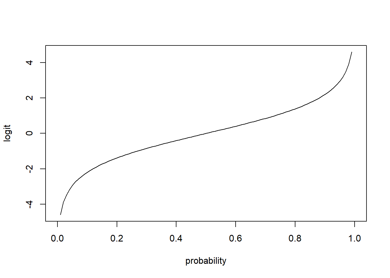

The inverse of the logit function is the sigmoid function: invlogit(logit(p)) = p

The inverse of the logit function maps real values to (0, 1).

\[invlogit(x) = \frac{exp(x)}{1+exp(x)} = \frac{1}{1+exp(-x)}\]

invlogit <- function(x){exp(x)/(1 + exp(x))}
x <- seq(-4, 4, 0.1)
plot(x, invlogit(x), type = "l", xlab = "logit", ylab = "probability")
abline(h = 0.5)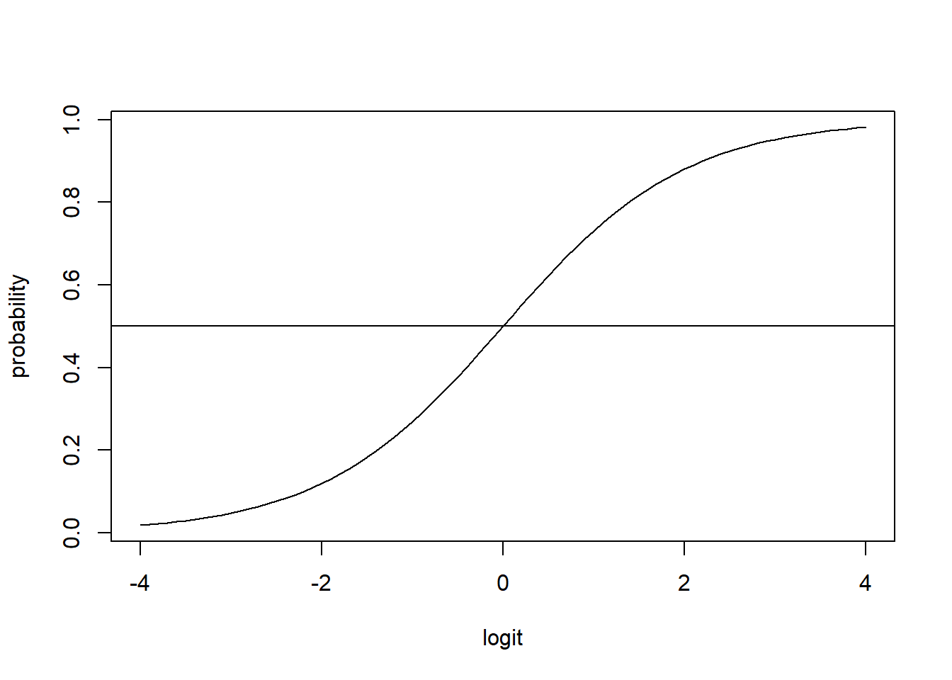

Binomial GLM with logit link is known as logistic regression model.

Canonical link function for Binomial data is the logit link.

\[logit(p) = \beta_0 + \beta_1 x_1 + \ldots + \beta_j x_j + \ldots + \beta_p x_p\]

If we increase \(x_j\) by one unit

\[logit(p^*) = \beta_0 + \beta_1 x_1 + \ldots + \beta_j (x_j+1) + \ldots + \beta_p x_p\]

\[logit(p^*) - logit(p) = \beta_j\]

\[\log\left(\frac{p^*}{1-p^*}\right) - \log\left(\frac{p}{1-p}\right) = \beta_j\]

\[\log\left(\frac{\frac{p^*}{1-p^*}}{\frac{p}{1-p}} \right) = \beta_j\] \[\mbox{Odds ratio (OR)}=\frac{\frac{p^*}{1-p^*}}{\frac{p}{1-p}} = exp(\beta_j)\]

Therefore,

\(\beta_j\) is the increase or decrease in the log-odds associated with one-unit increase in \(x_j\), holding all other variables constant

\[\log\left(\frac{p}{1-p}\ \ |_{x_j+1}\right)-\log\left(\frac{p}{1-p}\ \ |_{x_j}\right) = \beta_j\]

\(exp(\beta_j)\) is the odds ratio \[OR= \frac{\frac{p}{1-p}\ |_{x_j+1}} { \frac{p}{1-p} \ |_{x_j}} = exp(\beta_j)\]
When \(x_j\) increases one unit, the odds are multiplied by \(exp(\beta_j)\)

\[\frac{p}{1-p} |_{x_j+1} = \frac{p}{1-p} |_{x_j} \times exp(\beta_j)\]

Link function

The logit link function \(g(p)=\log(p/(1-p))\) is the canonical link function (logit makes the linear predictor \(\eta\) the same as the canonical parameter \(\theta\)).

The canonical link is not the only choice of link function. In the Binomial setting another common choice is the probit link function: \(g(p) = \Phi^{-1}(p)\) where \(\Phi\) is the standard normal cumulative distribution function.

24.1 Example binomial (1/0)

Example response variable disease or no disease

We use variable \(Y = 1\) if disease, \(Y = 0\) if no disease
\(p\) is the probability response variable \(Y = 1\) (disease)
\(\frac{p}{1-p}\) is the odds of disease

Consider the logistic model,

\[Y \sim Bernoulli(p)\]

\[\mbox{logit}(p)=\log(\mbox{odds})=\log\left(\frac{p}{1-p}\right)=\beta_0 + \beta_1 x_{1}\]

If we increase \(x_1\) by one unit,

\[\log\left(\frac{p^*}{1-p^*}\right)=\beta_0 + \beta_1 (x_{1}+1)\]

\[\log\left(\frac{p^*}{1-p^*}\right) - \log\left(\frac{p}{1-p}\right) = \beta_1\]

\[\frac{\frac{p^*}{1-p^*}}{\frac{p}{1-p}} = exp(\beta_1)\]

Therefore

\(\beta_1\) is the increase or decrease in the log-odds associated with one-unit increase in \(x_1\)

\[\log\left(\frac{p}{1-p}\ \ |_{x_1+1}\right)-\log\left(\frac{p}{1-p}\ \ |_{x_1}\right) = \beta_1\]

\(exp(\beta_1)\) is the odds ratio

\[OR= \frac{\frac{p}{1-p}\ |_{x_1+1}} { \frac{p}{1-p} \ |_{x_1}} = exp(\beta_1)\]

When \(x_1\) increases one unit, the odds are multiplied by \(exp(\beta_1)\)

\[\frac{p}{1-p} |_{x_1+1} = \frac{p}{1-p} |_{x_1} \times exp(\beta_1)\]

24.2 Example binomial (1/0)

In a Childhood Cancer case-control study, cases were ascertained as all children under ten years in England and Wales who died of cancer during 1954-1965. Exposure variable was whether or not the children received in utero irradiation. The year of birth was considered as a confounder of the association between irradiation and cancer.

Let \(p\) be the probability of being a case in the case-control study

XRAY = 1 if the child received in utero irradiation and 0 if not
BINYOB = 1 if YOB \(\geq 1954\) and 0 if YOB \(< 1954\)

\[logit(p) = \log(odds)=\log\left(\frac{p}{1-p}\right) = \beta_0 + \beta_1 XRAY + \beta_2 BINYOB\] \[\log(odds) = -0.061 + 0.501 XRAY + (-0.005)BINYOB\]

XRAY

0.501 is the increase of log(odds) of cancer for a person with XRAY = 1 versus another person with XRAY = 0, and with the same BINYOB.

The odds of cancer for a person with XRAY = 1 are exp(0.501)=1.65 times the odds of cancer of a person with XRAY = 0, and with the same BINYOB.

BINYOB

0.005 is the decrease of log(odds) of cancer for a person with BINYOB = 1 versus another person with BINYOB = 0, and with the same XRAY.

The odds of cancer for a person with BINYOB = 1 are exp(-0.005)=0.995 times the odds of cancer of a person with BINYOB = 0, and with the same XRAY.

24.3 Example binomial (grouped)

An experiment measures the toxicity of a pesticide to the tobacco budworm. Batches of 20 budworms of each sex were exposed to varying doses of the pesticide for three days and the number of budworms killed in each batch was recorded.

ldose <- rep(0:5, 2)
dead <- c(1, 4, 9, 13, 18, 20, 0, 2, 6, 10, 12, 16)
sex <- factor(rep(c("M", "F"), c(6, 6)))

data.frame(dead, ldose, sex)

   dead ldose sex
1     1     0   M
2     4     1   M
3     9     2   M
4    13     3   M
5    18     4   M
6    20     5   M
7     0     0   F
8     2     1   F
9     6     2   F
10   10     3   F
11   12     4   F
12   16     5   F

Logistic regression models can be fitted with glm() specifying family = "binomial". The logit link is the default for the binomial family so does not need to be specified.

Binomial responses can be specified as follows:

vector numeric 0/1 (0 = failure), logical (FALSE = failure), or factor (first level = failure)
two-column matrix with number of successes and number of failures

y <- cbind(dead, 20-dead)
y

      dead   
 [1,]    1 19
 [2,]    4 16
 [3,]    9 11
 [4,]   13  7
 [5,]   18  2
 [6,]   20  0
 [7,]    0 20
 [8,]    2 18
 [9,]    6 14
[10,]   10 10
[11,]   12  8
[12,]   16  4

y <- cbind(dead, 20-dead)

res <- glm(y ~ ldose + sex, family = "binomial")
summary(res)


Call:
glm(formula = y ~ ldose + sex, family = "binomial")

Coefficients:
            Estimate Std. Error z value Pr(>|z|)    
(Intercept)  -3.4732     0.4685  -7.413 1.23e-13 ***
ldose         1.0642     0.1311   8.119 4.70e-16 ***
sexM          1.1007     0.3558   3.093  0.00198 ** 
---
Signif. codes:  0 '***' 0.001 '**' 0.01 '*' 0.05 '.' 0.1 ' ' 1

(Dispersion parameter for binomial family taken to be 1)

    Null deviance: 124.8756  on 11  degrees of freedom
Residual deviance:   6.7571  on  9  degrees of freedom
AIC: 42.867

Number of Fisher Scoring iterations: 4

\[\log\left(\frac{p}{1-p}\right)= -3.47 + 1.061 \times \mbox{ldose} + 1.10 \times \mbox{sexM}\]

the odds of death for a male budworm are exp(1.10) = 3.01 times that for a female budworm, given a fixed dose of the pesticide.
the odds of death increase by a factor of exp(1.06) = 2.90 for every \(\mu\)g of pesticide, for male or female budworms.

Predictions

We can use the function predict(object, newdata, type, ...) to obtain predictions (?predict.glm):

object is the glm fitted object
newdata is a data frame with the variables with which to predict. If omitted, the fitted linear predictors are used.
type is type of prediction. When type = "link" predictions are on the scale of the linear predictors (log in the case of Poisson data, log-odds in the case of Binomial data). When type = "response" predictions are on the scale of the response variable (mean in the case of Poisson data, probabilities in the case of Binomial data).

Type "response" (probabilities):

# Predict at these dose levels
ld <- seq(0, 5, by = 0.1)
# Predict for males and dose levels seq(0, 5, by = 0.1)
newdataM <- data.frame(ldose = ld,
            sex = factor(rep("M", length(ld)), levels = levels(sex)))
# Predict for females and dose levels seq(0, 5, by = 0.1)
newdataF <- data.frame(ldose = ld,
            sex = factor(rep("F", length(ld)), levels = levels(sex)))

# Predictions for male and female
predictionsM <- predict(res, newdataM, type = "response")
predictionsF <- predict(res, newdataF, type = "response")

# Plot
plot(c(0, 5), c(0, 1), type = "n", xlab = "dose", ylab = "probability")
text(ldose, dead/20, as.character(sex))
lines(ld, predictionsM)
lines(ld, predictionsF)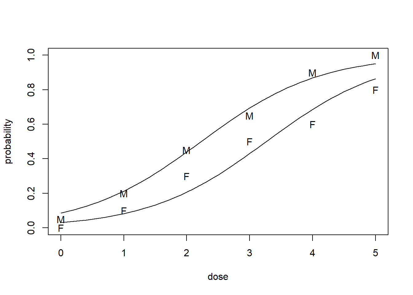

Type "link" (log-odds):

# Predict at these dose levels
ld <- seq(0, 5, by = 0.1)
# Predict for males and dose levels seq(0, 5, by = 0.1)
newdataM <- data.frame(ldose = ld,
            sex = factor(rep("M", length(ld)), levels = levels(sex)))
# Predict for females and dose levels seq(0, 5, by = 0.1)
newdataF <- data.frame(ldose = ld,
            sex = factor(rep("F", length(ld)), levels = levels(sex)))

# Predictions for male and female
predictionsM <- predict(res, newdataM, type = "link")
predictionsF <- predict(res, newdataF, type = "link")

# Plot
plot(c(0, 5), c(-4, 3), type = "n", xlab = "dose",ylab = "log(p/(1-p))")

lines(ld, predictionsM)
lines(ld, predictionsF)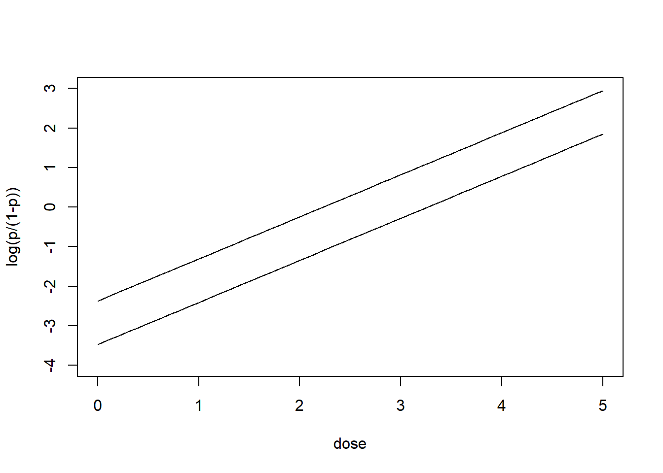

25 Modeling Normal data

The general linear model is a special case of GLM

Normal observations

\[Y_i \sim N(\mu_i, \sigma^2)\] Linear predictor

\[\eta_i = \beta_0 + \beta_1 x_{1i} + \ldots + \beta_p x_{pi}\]

Link function is the identity

\[g(\mu_i) = \mu_i\]

25.1 Example Normal data

Data on weekly food expenditure and household income for households with three family members.

d <- read.table("data/GHJ_food_income.txt", header = TRUE)
dim(d)

[1] 40  2

plot(d$Income, d$Food, xlab = "Weekly Household Income ($)",
ylab = "Weekly Household Food Expenditure ($)")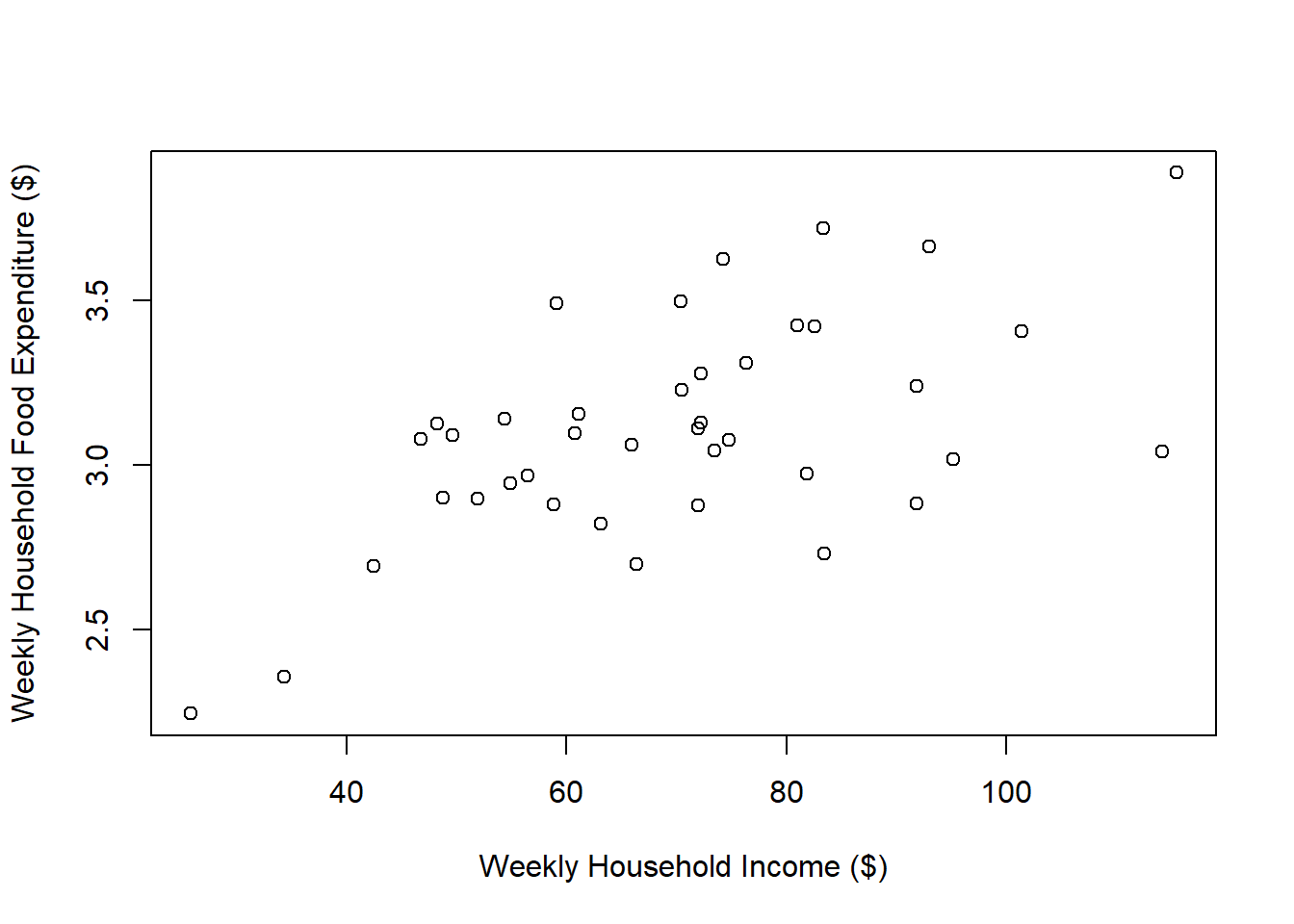

We first fit the model using lm(), then compare to the results using glm(). The default family for glm() is "gaussian" so the arguments of the call are unchanged.

foodLM <- lm(Food ~ Income, data = d)
summary(foodLM)


Call:
lm(formula = Food ~ Income, data = d)

Residuals:
     Min       1Q   Median       3Q      Max 
-0.50837 -0.15781 -0.00536  0.18789  0.49142 

Coefficients:
            Estimate Std. Error t value Pr(>|t|)    
(Intercept) 2.409418   0.161976  14.875  < 2e-16 ***
Income      0.009976   0.002234   4.465 6.95e-05 ***
---
Signif. codes:  0 '***' 0.001 '**' 0.01 '*' 0.05 '.' 0.1 ' ' 1

Residual standard error: 0.2766 on 38 degrees of freedom
Multiple R-squared:  0.3441,    Adjusted R-squared:  0.3268 
F-statistic: 19.94 on 1 and 38 DF,  p-value: 6.951e-05

foodGLM <- glm(Food ~ Income, data = d)
summary(foodGLM)


Call:
glm(formula = Food ~ Income, data = d)

Coefficients:
            Estimate Std. Error t value Pr(>|t|)    
(Intercept) 2.409418   0.161976  14.875  < 2e-16 ***
Income      0.009976   0.002234   4.465 6.95e-05 ***
---
Signif. codes:  0 '***' 0.001 '**' 0.01 '*' 0.05 '.' 0.1 ' ' 1

(Dispersion parameter for gaussian family taken to be 0.07650739)

    Null deviance: 4.4325  on 39  degrees of freedom
Residual deviance: 2.9073  on 38  degrees of freedom
AIC: 14.649

Number of Fisher Scoring iterations: 2

25.1.1 Coefficients

The estimated coefficients are the same. t-tests test the significance of each coefficient in the presence of the others.

25.1.2 Dispersion parameter

The dispersion parameter \(\phi \ (= \sigma^2)\) for the Gaussian family is estimated with the MSE \(\hat \sigma^2 = \sum (Y_i -\hat Y_i)^2/(n-p-1)\).

summary(foodLM)$sigma

[1] 0.2765997

summary(foodLM)$sigma^2

[1] 0.07650739

summary(foodGLM)$dispersion

[1] 0.07650739

25.1.3 Deviance

The deviance of a model is defined through the difference of the log-likelihoods between the saturated model (number of parameters equal to the number of observations) and the fitted model:

\[D = 2 \left( l({\boldsymbol{\hat\beta_{sat}}}) - l(\boldsymbol{\hat \beta}) \right) \phi,\]

\(l({\boldsymbol{\hat\beta_{sat}}})\) is the log-likelihood evaluated at the MLE of the saturated model, and \(l(\boldsymbol{\hat \beta})\) is the log-likelihood evaluated at the MLE of the fitted model.

The scaled deviance is obtained by dividing the deviance by the dispersion parameter

\[D^* = D/\phi = 2 \left( l({\boldsymbol{\hat\beta_{sat}}})- l(\boldsymbol{\hat \beta}) \right)\]

If \(\phi=1\) such as in the binomial or Poisson regression models, then both the deviance and the scaled deviance are the same.

The scaled deviance has asymptotic chi-squared distribution with degrees of freedom equal to the change in number of parameters in the models.

\[D^* \sim \chi^2_{n-p-1}\]

Example

For Gaussian data, the deviance is equal to the residual sum of squares RSS.

\[D = RSS = \sum (Y_i - \hat Y_i)^2\]

In the Gaussian model:

\[D^* = \frac{D}{\phi} = \frac{RSS}{\sigma^2} = \frac{\sum_{i=1}^n(Y_i - \hat Y_i)^2}{\sigma^2} \mbox{ is distributed as a } \chi^2_{n-p-1}\]

Null deviance and Residual deviance

The R output shows the deviance of two models:

Null deviance

Null deviance defined through is the difference of the log-likelihoods between the saturated model and the null model (model with just an intercept). Degrees of freedom \(n-1\), where \(n\) is the number of observations and 1 comes from the intercept.

Residual Deviance

Residual deviance defined through the difference of the log-likelihoods between the saturated model and the fitted model. Degrees of freedom \(n − p - 1\), where \(p\) is the number of explanatory variables and 1 comes from the intercept.

25.1.4 Akaike Information Criterion (AIC)

The AIC is a measure of fit that penalizes for the number of parameters \(p\)

\[AIC = -2 \mbox{log-likelihood} + 2(p+1)\] where \(\mbox{log-likelihood}\) is the maximized log likelihood of the model and \(p+1\) the number of model parameters including the intercept.

Smaller values indicate better fit and thus the AIC can be used to compare models (not necessarily nested).