5 ANOVA

Learning objectives

ANOVA
Calculate ANOVA table
Tukey test
t test and ANOVA for comparing two samples
Multiple comparisons

5.1 ANOVA

ANOVA (also known as Analysis of Variance) is a statistical procedure to test if the means of two or more groups are significantly different from each other.

We can use ANOVA to study the effect of different levels of a variable on a response (e.g., study the effect of four different treatments for pain on the mean time to pain relief, the effect of three different levels of a fertilizer on mean plant growth, or the effect of five machines on the mean time to complete a given task).

5.1.1 Null and alternative hypothesis

In ANOVA, the null hypothesis is all the population means are equal (there is not relationship between explanatory variable and response). The alternative hypothesis is population means are not all equal, that is, at least two population means are different from each other (there is a relationship between explanatory variable and response).

\(H_0: \mu_1 = \mu_2 = \ldots = \mu_k\)
\(H_1:\) not all \(\mu_i\) are equal

ANOVA is an extension of the independent two-samples t-test for comparing means when there are more than two groups.

5.1.2 Variability

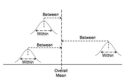
ANOVA separates the total variation in the data into variation between groups and variation within groups.

5.1.3 F statistic

ANOVA uses a test statistic called F statistic that compares the variability between groups to the variability within groups.
\[\mbox{F = between groups variability / within groups variability}\] If the variability between groups dominates the variability within groups, we find evidence to suggest population means are different.

5.1.4 Assumptions

ANOVA is based in three assumptions:

Independence. All samples are drawn independently of each other. Within each sample, the observations are sampled randomly and independently of each other
Normality. The observations are approximately normal
Equal variances. The variances of the populations are equal

5.2 Variability

ANOVA separates the total variation in the data into variation between groups and variation within groups.

\[\mbox{SST = SSB + SSW}\]

Let us define

\(k\) number of groups
\(n\) total sample size (all groups combined)
\(n_k\) sample size of group \(k\)
\(\bar x_k\) sample mean of group \(k\)
\(\bar x\) grand mean (i.e., mean for all groups combined)

Then

Grand mean:
\[\bar x = \frac{\sum_k \sum_i x_{ik}}{n}\]
Total variation:
\[\mbox{SST} = \sum_k \sum_i (x_{ik}-\bar x)^2\] Sum of squares of the differences between the data and the grand mean.
It measures variation of the data around the grand mean.
Between group variation:
\[\mbox{SSB} = \sum_k n_k(\bar x_k-\bar x)^2\] Sum of squares of the differences between the group means and the grand mean.
It measures variation of the group means around the grand mean.
Within group variation:
\[\mbox{SSW} = \sum_k \sum_i (x_{ik}-\bar x_{k})^2\]
Sum of squares of the differences between the data and the group means.
It measures variation of each observation around its group mean \(\bar x_k\).

5.3 F statistic

ANOVA uses a test statistic called F statistic that compares the variability between groups to the variability within groups. That is, compares how much individuals in different groups vary from one another over how much individuals within groups vary from one another.

\[F = \frac{\sum_k n_k(\bar x_k-\bar x)^2/(k-1)}{\sum_k \sum_i (x_{ik}-\bar x_{k})^2/(n-k)} = \frac{SSB/(k-1)}{SSW/(n-k)} = \frac{MSB}{MSW} \sim F(k-1, n-k)\]

The sampling distribution of the F statistic is the F distribution with degrees of freedom \(k-1\) (number of groups - 1) and \(n-k\) (number of observations - number of groups).

If the sample means are close to each other (and therefore to the grand mean) SSB will be small.
If the between variation is larger than the within variation, the F statistic is large (F > 1), and there is evidence to suggest the population means are not the same.
If the between and within variation are similar, the F statistic is small (F \(\approx\) 1), and there is not evidence to suggest population means are not the same.

5.4 Example ANOVA

Consider an experiment to compare plant yields under a control and two different treatment conditions. We collect the dried weight of plants for the control group and the two treatments. We use ANOVA to test whether the average plant weights for each treatment are statistically different from each other.

d <- PlantGrowth
d

   weight group
1    4.17  ctrl
2    5.58  ctrl
3    5.18  ctrl
4    6.11  ctrl
5    4.50  ctrl
6    4.61  ctrl
7    5.17  ctrl
8    4.53  ctrl
9    5.33  ctrl
10   5.14  ctrl
11   4.81  trt1
12   4.17  trt1
13   4.41  trt1
14   3.59  trt1
15   5.87  trt1
16   3.83  trt1
17   6.03  trt1
18   4.89  trt1
19   4.32  trt1
20   4.69  trt1
21   6.31  trt2
22   5.12  trt2
23   5.54  trt2
24   5.50  trt2
25   5.37  trt2
26   5.29  trt2
27   4.92  trt2
28   6.15  trt2
29   5.80  trt2
30   5.26  trt2

The groups are control, treatment 1 and treatment 2.

levels(d$group)

[1] "ctrl" "trt1" "trt2"

For each group, we calculate the number of observations and the means and standard deviations of weights. We observe mean weights are different between groups. Are the mean weights statistically different or are just different due to sampling variability?

print(aggregate(d$weight, by = list(d$group),
          FUN = function(x){c(length = length(x), mean = mean(x), sd = sqrt(var(x)))}))

  Group.1   x.length     x.mean       x.sd
1    ctrl 10.0000000  5.0320000  0.5830914
2    trt1 10.0000000  4.6610000  0.7936757
3    trt2 10.0000000  5.5260000  0.4425733

The boxplot shows means are different. It also shows each group present different amount of variation in the response and there is overlap between groups.

boxplot(weight ~ group, data = d)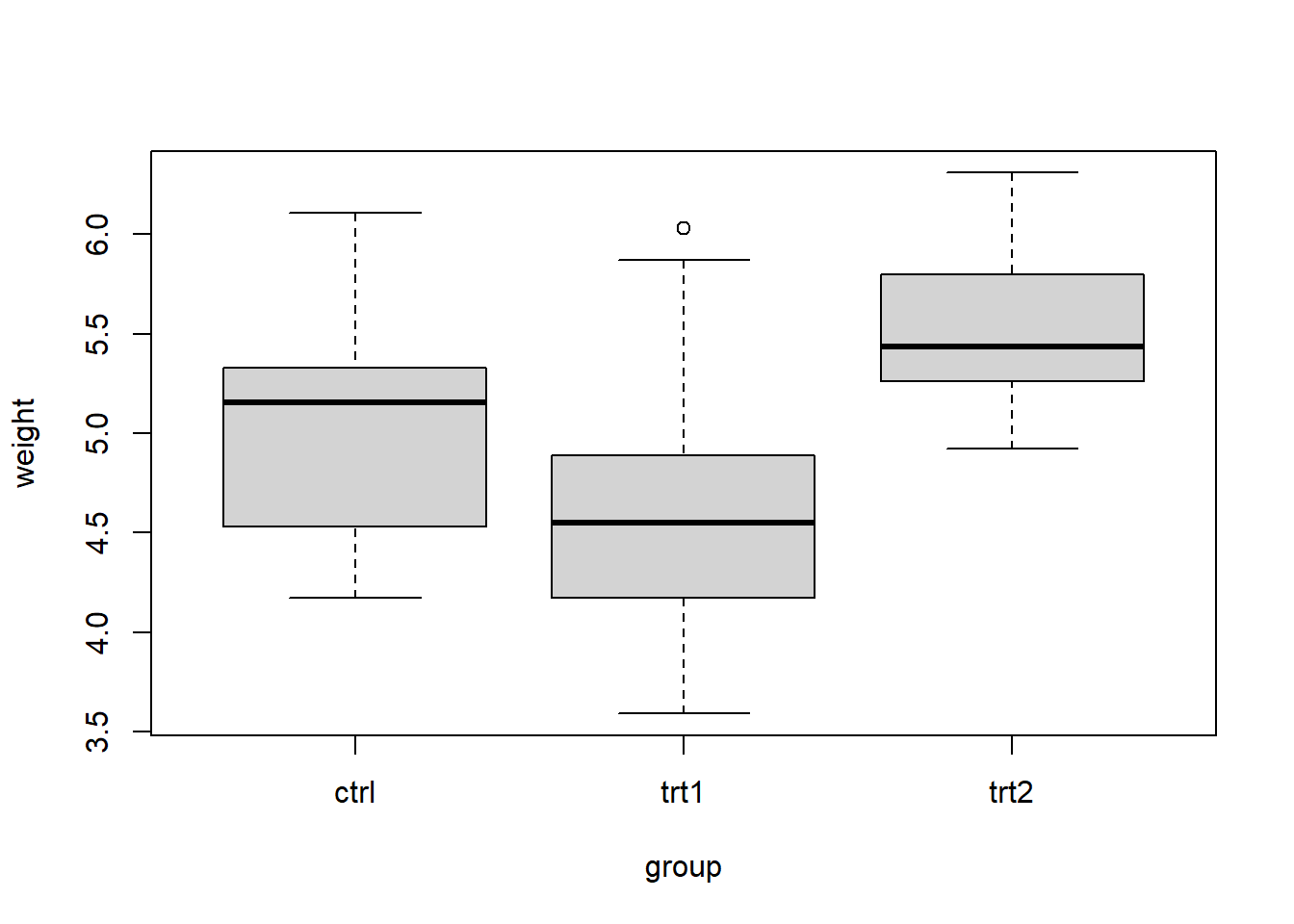

We use ANOVA to test if the weight means for each treatment are statistically different or are just different due to sampling variability.

Null and alternative hypotheses
\(H_0: \mu_1 = \mu_2 = \mu_3\)
\(H_1:\) At least one population mean is different
We set the significance level
\(\alpha = 0.05\)
F statistic
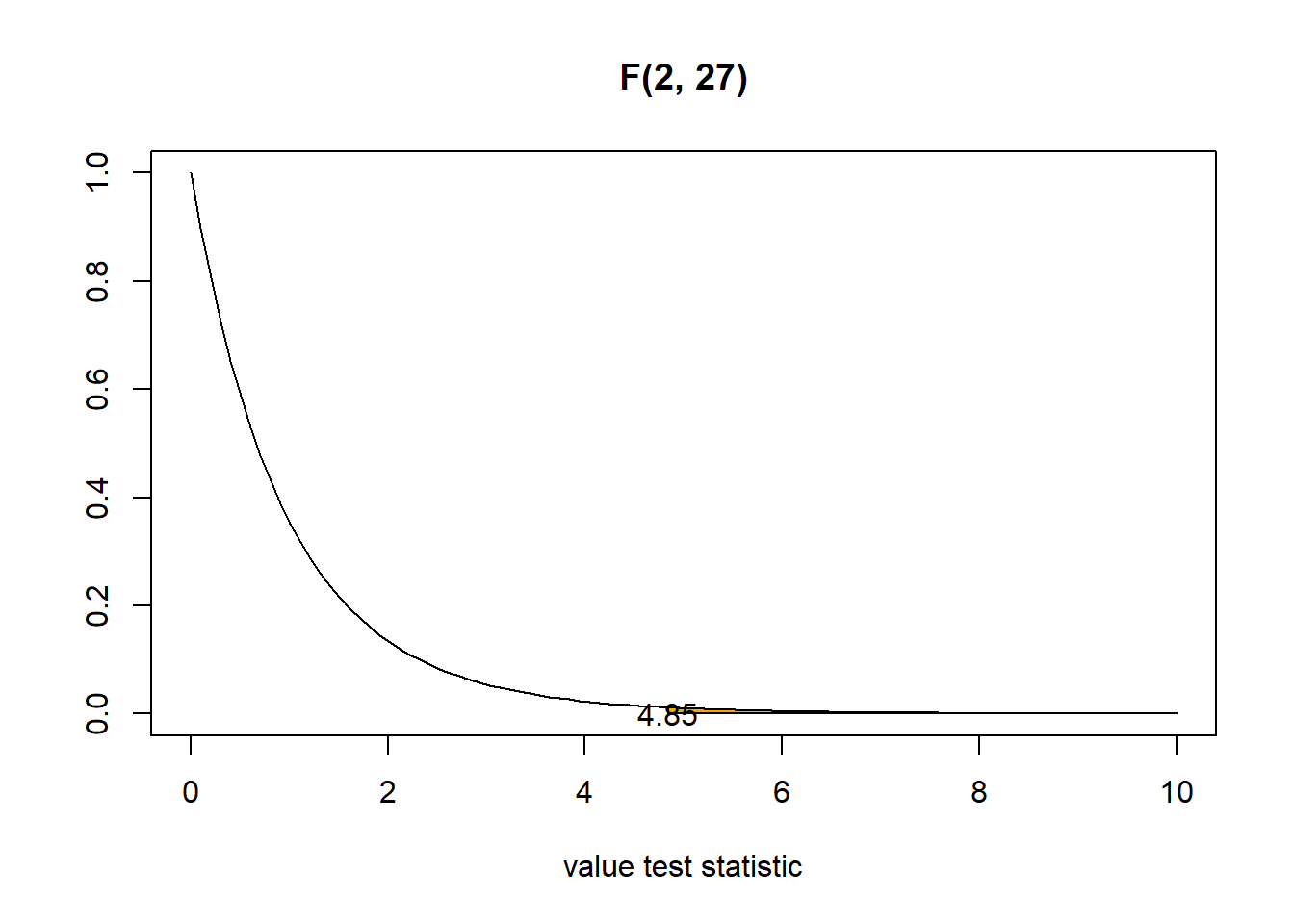
F statistic compares the variation between groups to the variation within groups. \[F = \frac{SSB/(k-1)}{SSW/(n-k)} = \frac{MSB}{MSW} \sim F(k-1, n-k) = F(3-1, 30-3)\]

We conduct ANOVA with the aov() function and get F statistic = 4.85.

res <- aov(weight ~ group, data = d)
summary(res)

            Df Sum Sq Mean Sq F value Pr(>F)  
group        2  3.766  1.8832   4.846 0.0159 *
Residuals   27 10.492  0.3886                 
---
Signif. codes:  0 '***' 0.001 '**' 0.01 '*' 0.05 '.' 0.1 ' ' 1

The p-value is the probability of obtaining a F-statistic equal to the one observed or more extreme, under the null distribution. If the F statistic observed is large (variation between different groups is larger than the variation within groups), the p-value will be small.

Here the p-value is the area under the F(2,27) curve to the right of the F statistic observed (4.85). The p-value is 0.016.

Decision
If p-value < \(\alpha\), we reject the null.
If p-value \(\geq \alpha\), we fail to reject the null.

Here, p-value \(< \alpha\) (0.016 < 0.05) , so we reject the null. We conclude there is evidence that at least two of the group means are different.

5.5 ANOVA table

Source	SS	df	MS	F	P
Between(Group)	SSB	k-1	MSB=SSB/(k-1)	MSB/MSW	P
Within(Error)	SSW	n-k	MSW=SSW/(n-k)
Total	SST	n-1

\[\mbox{SST = SSB + SSW}\]

SS: Sum of Squares (Sum of Squares of the deviations)

SSB = \(\sum_k n_k(\bar x_k-\bar x)^2\) variation BETWEEN groups.
SSW = \(\sum_k \sum_i (x_{ik}-\bar x_{k})^2\) variation WITHIN the groups or unexplained random error.
SST = \(\sum_k \sum_i (x_{ik}-\bar x)^2\) TOTAL variation in the data from the grand mean.

df: Degrees of freedom

Degrees of freedom of SSB = \(k-1\). Variation of the \(k\) group means about the overall mean
Degrees of freedom of SSW = \(n-k\). Variation of the \(n\) observations about \(k\) group means
Degrees of freedom of SST = \(n-1\). Variation of all \(n\) observations about the overall mean

\[n-1 = (k-1)+(n-k)\]

The total variance of observed data can be expressed as the total sum of squares divided by the total degrees of freedom: \[s^2=\sum_k \sum_i (x_{ik}-\bar x)^2/(n-1) = SST/DFT\]

MS: Mean Squares

MS = SS/df

F: F-statistic

F-statistic = MSB/MSW

Assuming the null hypothesis is true, the F statistic has an F(k-1, n-k) distribution.

P: p-value

The p-value is the probability of observing a F-statistic as the one observed or more extreme under the null distribution.
The null is rejected if the F observed is sufficiently large.

Example

The following ANOVA table is partially completed.

Source	DF	SS	MS
Between groups	?	258	?
Within groups	26	?	?
Total	29	898

Complete the table.
How many groups were there in the study?
How many total observations were there in the study?

Solution

df(B) = 29-26=3
SSW = 898-258=640
MSB = 258/3 = 86
MSW = 640/26 = 24.61

df(B) = k-1 = 3 Thus, 4 groups
df(W) = n-k = 26
df(T) = n-1 = 29 Thus, 30 observations

The following ANOVA table is only partially completed.

Source	DF	SS	MS
Between groups	3	?	45
Within groups	12	337	?
Total	?	472

Complete the table.
How many groups were there in the study?
How many total observations were there in the study?

Solution

df(T) = 3+12=15
SSB = 472-337=135
MSB = 135/3 = 45
MSW = 337/12 = 28.08

df(B) = k-1 = 3 Thus, 4 groups
df(W) = n-k = 12
df(T) = n-1 = 15 Thus, 16 observations

5.6 Manually calculating ANOVA table

We can obtain the ANOVA table with the aov() function. Here we show how to manually calculate the ANOVA table for the example of plant growth data.

SS: Sum of Squares (Sum of Squares of the deviations)

\[\mbox{SST = SSB + SSW}\]

SSB = \(\sum_k n_k(\bar x_k-\bar x)^2\) variation BETWEEN groups.
SSW = \(\sum_k \sum_i (x_{ik}-\bar x_{k})^2\) variation WITHIN the groups or unexplained random error.
SST = \(\sum_k \sum_i (x_{ik}-\bar x)^2\) TOTAL variation in the data from the grand mean.

# Grand mean
barx <- mean(d$weight)

# SST
SST <- sum((d$weight - barx)^2)

# SSB
# Compute the mean of each group
meangroups <- aggregate(d$weight, list(d$group), mean)$x
# Compute the size of each group
sizegroups <- aggregate(d$weight, list(d$group), length)$x
SSB <- sum(sizegroups*(meangroups - barx)^2)

# SSW
SSW <- SST - SSB

SSB

[1] 3.76634

SSW

[1] 10.49209

SST

[1] 14.25843

df: Degrees of freedom

Degrees of freedom of SSB = \(k-1\). Variation of the \(k\) group means about the overall mean
Degrees of freedom of SSW = \(n-k\). Variation of the \(n\) observations about \(k\) group means
Degrees of freedom of SST = \(n-1\). Variation of all \(n\) observations about the overall mean

\[n-1 = (k-1)+(n-k)\]

# number groups
num_groups <- length(unique(d$group))
# number observations
num_obs <- length(d$weight)

# df numerator k-1
df1 <- num_groups - 1
# df denominator n-k
df2 <- num_obs - num_groups

df1

[1] 2

df2

[1] 27

MS: Mean Squares

MS = SS/df

MSB <- SSB/df1
MSW <- SSW/df2
MSB

[1] 1.88317

MSW

[1] 0.3885959

F: F-statistic

F-statistic = MSB/MSE

F_obs <- MSB/MSW
F_obs

[1] 4.846088

p-value

Probability under the F(k-1, n-k) distribution greater than the oberved F statistic

p <- 1 - pf(q = F_obs, df1 = df1, df2 = df2)
p

[1] 0.01590996

5.7 Assumptions

Assumptions in ANOVA are independence, normality and equal variances. We check the assumptions for the example of plant growth data.

5.7.1 Independence

Independence. All samples are drawn independently of each other. Within each sample, observations are sampled randomly and independently of each other

5.7.2 Normality

Normality. The observations are approximately normal

We can use the Shapiro-Wilk test to determine whether the observations are normally distributed

\(H_0\): observations are normal
\(H_1\): observations are not normal

shapiro.test(d$weight)


    Shapiro-Wilk normality test

data:  d$weight
W = 0.98268, p-value = 0.8915

\(\alpha = 0.05\), test statistic = 0.98268, p-value = 0.8915

p-value > \(\alpha\), we fail to reject the null hypothesis. We can assume normality

Moreover, note that ANOVA is relatively robust to violations of normality provided:

The populations are symmetric and uni-modal
The sample sizes for the groups are equal or greater than 10

5.7.3 Equal variances

Equal variances. The variances of the populations are equal

We can use Levene’s test to check homogeneity of variances

\(H_0:\) variances are equal
\(H_1:\) variances are not equal

library(car)

Loading required package: carData

leveneTest(weight ~ group, data = d)

Levene's Test for Homogeneity of Variance (center = median)
      Df F value Pr(>F)
group  2  1.1192 0.3412
      27

\(\alpha = 0.05\), test statistic = 1.1192, p-value = 0.3412

p-value \(> \alpha\), we fail to reject the null hypothesis. There is not evidence to suggest that variance across groups is statistically different. Therefore we can assume the homogeneity of variances in the different groups.

A general rule of thumb for equal variances is to compare the largest and smallest sample variances. If the ratio of largest to smallest variance is smaller than 3, then it may be that the assumption is not violated.

5.8 Tukey multiple pairwise-comparisons

In ANOVA, we test whether some of the group means are different. However, if the results are significant, we do not know which pairs of means are different.

We can perform a Tukey test to perform multiple pairwise-comparisons and determine if the mean difference between specific pairs of group are statistically significant.

We can use the function TukeyHSD() (Tukey’s ‘Honest Significant Difference’).

TukeyHSD(res)

  Tukey multiple comparisons of means
    95% family-wise confidence level

Fit: aov(formula = weight ~ group, data = d)

$group
            diff        lwr       upr     p adj
trt1-ctrl -0.371 -1.0622161 0.3202161 0.3908711
trt2-ctrl  0.494 -0.1972161 1.1852161 0.1979960
trt2-trt1  0.865  0.1737839 1.5562161 0.0120064

The output shows the following:

diff is the difference between means of the two groups
lwr, upr are the lower and the upper limits of 95% confidence intervals, respectively
p adj is the p-value after adjustment for multiple comparisons

In this example the output shows that the only significant difference is between group trt2 and trt1 (p-value = 0.012). The confidence interval for trt2 - trt1 does not include 0. So we reject the null hypothesis that there is no difference in group trt2 and trt1 means.

5.9 t tests

ANOVA is used to compare the means of two or more than two populations. The t-test is used to compare the means of two populations.

When we only have two groups ANOVA and the t-test give the same results.

Example

Suppose we want to test whether the average women’s weight differs from the average men’s weight.

\(H_0: \mu_w = \mu_m\)
\(H_1: \mu_w \neq \mu_m\)

We take a sample with the weights of 18 individuals (9 women and 9 men).

women_weight <- c(41.5, 59.3, 73.3, 69.5, 46.2, 41.5, 26.3, 33.4, 65)
men_weight <- c(65.9, 55.8, 67.5, 65.5, 71.1, 89.1, 58.9, 66.8, 65.2)
d <- data.frame(group = rep(c("Woman", "Man"), each = 9),
                weight = c(women_weight, men_weight))

ANOVA

summary(aov(weight ~ group, data = d))

            Df Sum Sq Mean Sq F value Pr(>F)  
group        1   1247  1246.7    6.81  0.019 *
Residuals   16   2929   183.1                 
---
Signif. codes:  0 '***' 0.001 '**' 0.01 '*' 0.05 '.' 0.1 ' ' 1

The test statistic is F = Between groups variability / Within groups variability = 6.81 \[F = MSB/MSW \sim F(k-1, n-k)\]

The p-value is 0.019 so we reject the null

t-test

We assume that the two samples are drawn from populations with identical population variances. The test statistic is calculated as

\[T = \frac{(\bar X_1 - \bar X_2) - 0}{\sqrt{\frac{S_p^2}{n_1}+\frac{S_p^2}{n_2} }} \sim t(n_1+n_2-2)\]

where \(S_p^2\) is an estimator of the pooled variance of the two groups.

\[S_p^2 = \frac{(n_1-1)S_1^2 + (n_2-1)S_2^2 }{n_1+n_2-2}\]

n1 <- 9
x1 <- mean(women_weight)
s1 <- var(women_weight)

n2 <- 9
x2 <- mean(men_weight)
s2 <- var(men_weight)

sp <- ((n1-1)*s1 + (n2-1)*s2)/(n1+n2-2)

t <- (x1-x2)/sqrt(sp/n1 + sp/n2)
t

[1] -2.609519

The p-value is the probability that observing a test statistic equal to -2.6 or more extreme (in both directions) in the null distribution

df <- min(n1+n2-2)
2*pt(t, df)

[1] 0.01897032

The p-value is 0.019 so we reject the null.

We can also conduct the test with the function t.test() with var.equals = TRUE to treat the two variances as being equal. In this case, the pooled variance is used to estimate the variance.

t.test(women_weight, men_weight, var.equal = TRUE)


    Two Sample t-test

data:  women_weight and men_weight
t = -2.6095, df = 16, p-value = 0.01897
alternative hypothesis: true difference in means is not equal to 0
95 percent confidence interval:
 -30.165960  -3.122929
sample estimates:
mean of x mean of y 
 50.66667  67.31111

Note that \(t_{df}^2 = F(1,df)\) ((-2.61^2)=6.81) and the p-values and therefore the conclusions are identical for both tests. p-value < \(\alpha\) (0.019 < 0.05), we reject the null hypothesis and conclude there is evidence to support the average weights in women and men are different.

5.10 Multiple pairwise-comparisons

When we have more than two groups, we have seen we can use ANOVA to test whether the group means are different from each other, and the Tukey test to find out which pairs of groups are different.

We can think we could also conduct multiple two independent t-tests for comparing two samples. But the problem with this approach is that the significance levels can be misleading.

Suppose we have \(k\) groups and we perform multiple independent t-tests for pairwise comparisons of two means. In this case we would need to perform \(\frac{k!}{(k-2)!2!}\) tests (number of combinations of \(k\) groups taken 2 at a time). For example, if \(k\)=10 groups, we need to perform \(\frac{10!}{(10-2)!2!} = 45\) independent t-tests.

If we used a significance level of 0.05, the probability of observing at least one significant result when there is no differences between groups is \[P(\mbox{at least one significant result|no differences}) =\] \[= 1 - P(\mbox{no significant results|no differences}) = 1 - (1-0.05)^{45} = 0.90\] (Remember \(P(\mbox{reject } H_0 |H_0 \mbox{ is true}) = \alpha\) and \(P(\mbox{not reject} H_0 |H_0 \mbox{ is true}) = 1 - P(\mbox{reject} H_0 |H_0 \mbox{ is true}) = 1 - \alpha\)).

Therefore, if we consider 45 tests and a significance level of 0.05, we have a probability of 0.90 of observing at least one significant result, even if there are no differences.

This shows multiple t-tests would lead to a greater chance of making a Type I error.

Methods for dealing with multiple testing often adjust \(\alpha\) in some way, so that the probability of observing at least one significant result due to chance remains below the desired significance level.

When comparing more than two groups we use ANOVA because this avoids increasing the likelihood of a Type I error.