14 Unusual observations
Occasionally, a few observations may not fit the model well. These have the potential to dramatically alter the results, so we should check for them and investigate their validity.
We should always check fitted models to make sure that these assumptions have not been violated. Diagnostic methods are based primarily on the residuals. Residual analysis is usually done graphically. We may look at quantile plots to assess normality, and scatterplots to assess assumptions such as constant variance and linearity, and to identify potential outliers.
14.1 Unusual observations
Outlier (unusual \(y\)): observation whose response value \(y\) does not follow the general trend of the rest of the data. Outliers have standardized residual less than -2 or greater than 2 (or -3 and 3). The bigger the data set, the more outliers we expect to get, about 5% of the sample.
High leverage observation (unusual \(x\)): observation that has extreme predictor \(x\) values. With a single predictor, an extreme \(x\) value is simply one that is particularly high or low compared with all the other data observations. With multiple predictors, extreme \(x\) values may be particularly high or low for one or more predictors, or may be “unusual” combinations of predictor values (e.g., with two predictors that are positively correlated, an unusual combination of predictor values might be a high value of one predictor paired with a low value of the other predictor). An observation is usually considered to have high leverage if it has leverage (“hat”) greater than 2 times the average of all leverage values. That is, if \(h_{ii} > 2(p+1)/n\).
Influential observation: An observation is influential if its omission causes statistical inference to change, such as the predicted responses, the estimated slope coefficients, or the hypothesis test results. Cook’s distance combines residuals and leverages in a single measure of influence. We usually say an observation is influential is Cook’s distance is greater than \(4/n\), where \(n\) is the sample size. We should examine in closer detail the points with values Cook’s distance that are substantially larger than the rest.
It is possible for an observation to be both an outlier and have high leverage.
Influential observations can be outliers, leverage observations or both. But an outlier or leverage observation may not be influential.
Outliers and high leverage data points have the potential to be influential, but we generally have to investigate further to determine whether or not they are actually influential.
14.1.1 Examples unusual observations
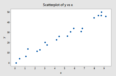
Example 1
All of the data points follow the general trend of the rest of the data, so there are no outliers (unusual \(y\)). And, none of the data points are extreme with respect to \(x\), so there are no high leverage points. Overall, none of the data points appear to be influential with respect to the location of the best fitting line.
Example 2
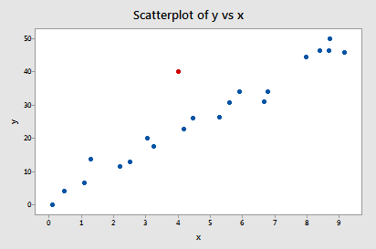
Because the red point does not follow the general trend of the rest of the data, it would be considered an outlier. However, this point does not have an extreme \(x\) value, so it does not have high leverage.
Is the red data point influential? An easy way to determine if the data point is influential is to find the best fitting line twice - once with the red data point included and once with the red data point excluded.
The predicted responses, estimated slope coefficients, and hypothesis test results are not affected by the inclusion of the red data point. Therefore, the data point is not deemed influential. In summary, the red data point is not influential and does not have high leverage, but it is an outlier.
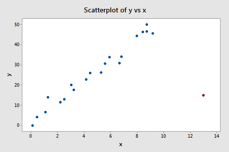
Example 3
In this case, the red point follows the general trend of the rest of the data. Therefore, it is not deemed an outlier. However, this point does have an extreme \(x\) value, so it does have high leverage.
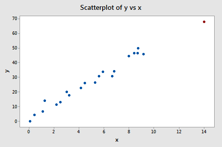
Is the red data point influential? It certainly appears to be far removed from the rest of the data (in the \(x\) direction), but is that sufficient to make the data point influential in this case?
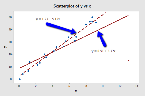
The predicted responses, estimated slope coefficients, and hypothesis test results are not affected by the inclusion of the red data point. Therefore, the data point is not deemed influential. In summary, the red data point is not influential, nor is it an outlier, but it does have high leverage.
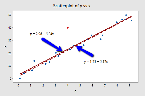
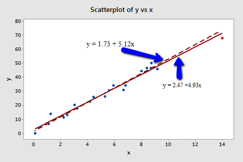
Example 4
The red data point is certainly an outlier and has high leverage. The red data point does not follow the general trend of the rest of the data and it also has an extreme \(x\) value.
In this case the red data point is influential. The two best fitting lines - one obtained when the red data point is included and one obtained when the red data point is excluded are substantially different. The solid line represents the estimated regression equation with the red data point included, while the dashed line represents the estimated regression equation with the red data point taken excluded.
14.2 Unusual observations
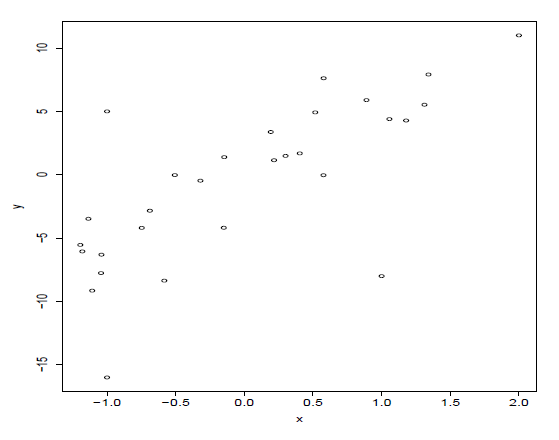
Below is a scatter plot for a data set. Identify the outliers in the data set. Which of \(R^2\), \(\hat \sigma\), \(se(\hat \beta_1)\) and the t-value for testing \(H_0: \beta_1 = 0\) would change if you drop these outliers (all of them at once)? Justify your answers.
Unusual observations. Solutions
Outlier 1: (x,y)=(1,-9). Outlier 2: (x,y)=(-1,5). Outlier 3: (x,y)=(-1,-16). The observation at (2, 10) is high leverage.
If you drop all outliers, the \(R^2\) would increase (better fit) and \(\hat \sigma\) would decrease.
\(t = \frac{\hat \beta_1}{se(\hat \beta_1)},\ \ se(\hat \beta_1) = \hat \sigma \sqrt{ (X'X)^{-1}_{11} }\)
The slope would probably increase a bit without the outliers so the numerator in the t-test would increase. The SE would decrease somewhat (depending on how much \(\hat \sigma\) decreases compared to the sample size reduction) and so the t would increase.