25 Survival analysis

25.1 Introduction

Survival analysis is a collection of statistical procedures for data analysis for which the outcome variable of interest is time until an event occurs.

By event, we mean death, disease incidence, relapse from remission, recovery or any designated experience of interest that may happen to an individual.

We refer to the time variable as survival time, because it gives the time that an individual has “survived” over some follow-up period. We also refer to the event as a failure, because the event of interest usually is death, disease incidence, or some other negative individual experience. However, survival time may be “time to return to work after an elective surgical procedure”, in which case failure is a positive event.

Examples of events:

Cancer patients/ time until tumor recurrence
Disease-free cohort / time until heart disease (years)
Elderly (60+) population / time until death (years)
Heart transplants / time until death (months)
Machines / time until a machine part fails
HIV patients/ time until AIDS

Sometimes we are interested in

Estimating and interpreting survival functions
Comparing survival functions
Assessing how a risk factor or treatment affects time to disease or some other event (e.g., assess the relationship of explanatory variables to survival time)

25.1.1 Censoring

The survival time response may be incompletely determined for some subjects. For example, for some subjects we may know that their survival time was at least equal to some time \(t\). Whereas, for other subjects, we will know their exact time of event. Incompletely observed responses are censored.

Censoring is present when we have some information about a subject’s event time, but we do not know the exact event time. For the analysis methods we will discuss to be valid, censoring mechanism must be independent of the survival mechanism.

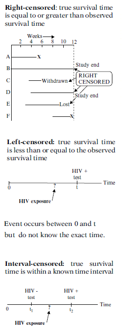
There are generally three reasons why censoring might occur:

A subject does not experience the event before the study ends
A person is lost to follow-up during the study period
A person withdraws from the study

These are all examples of right-censoring.

Left-censored. We know HIV+ occurred between 0 and \(t\) (\(t\) is the time when HIV test was done) but we do not know the exact time.

Interval-censored. We know HIV+ occurred between \(t_1\) (time when HIV was done and was negative) and \(t_2\) (time when HIV test was done and was positive) but we do not know the exact time.

25.1.2 Survival data

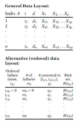
General data layout:

First column identifies the study subjects.
Second column gives the observed survival times.
Third column is the dichotomous variable that indicates censorship status (1 failed/0 censored).
The remainder of the information in the table gives values for explanatory variables of interest.

Alternative data layout:

First column gives ordered survival times (failures only, not censored times) from smallest to largest. Table begins with a survival time 0 in case some subjects have been censored before the first failure time.
Second column gives frequency counts of failures at each distinct failure time.
Third column gives frequency counts, denoted by \(q_f\), of those persons censored in the time interval starting with failure time \(t_{(f)}\) up to but not including the next failure time, denoted by \(t_{(f+1)}\).
Last column gives the risk set, which denotes the number of individuals who have survived at least to time \(t_{(f)}\) (failure may be at \(t_{(f)}\) of after).

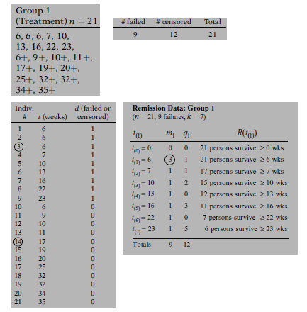
Example:

Survival times of 21 individuals. In the table, 6 means observed survival time is 6 and is not censored, 6+ means survival time is 6 and is censored

25.2 Survival time distribution

There are several equivalent ways to characterize the probability distribution of a survival time random variable \(T\geq 0\).

The survival function \(S(t)\)
The hazard function \(h(t)\)
The probability density function \(f(t)\)
The cumulative distribution function \(F(t)\)
The cumulative hazard function \(H(t)\)

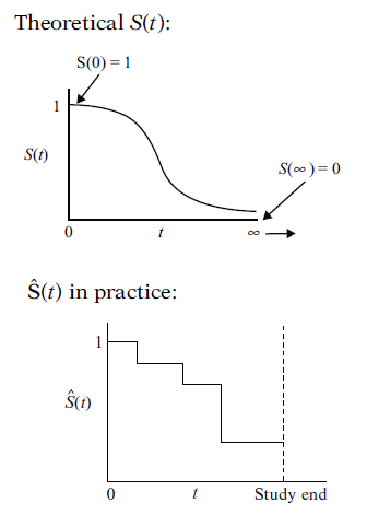
Survival function S(t)

The survival function gives the probability that a subject will survive past time \(t\).

\[S(t) = P(T > t),\ t \geq 0\]

\(S(0) = 1\). That is, the probability of surviving past time 0 is 1.
\(lim_{t \rightarrow \infty}S(t) = 0\). As time goes to infinity, the survival curve goes to 0.
The function then decreases (or remains constant) over time, and never drops below 0.
In theory, the survival function is smooth. In practice, we observe events on a discrete time scale (days, weeks, etc.).

Hazard function h(t)

The hazard function (also known as the intensity function or the force of mortality) is the instantaneous rate at which events occur, given no previous events.

It is the probability that, given that a subject has survived up to time \(t\), they fails in the next small interval of time, divided by the length of that interval.

\[h(t) = lim_{\Delta t \rightarrow 0} \frac{P(t < T \leq t + \Delta t\ |\ T > t)}{\Delta t}\]

Cumulative distribution function (CDF) F(t)

The cumulative distribution function (CDF) (also known as the cumulative risk function) is given by \[F(t) = P(T \leq t)\] This is the complement of the survival function: \[S(t) = P(T > t) = 1- P(T \leq t) = 1 - F(t)\]

Probability density function (PDF) f(t)

The probability density function (PDF) is the rate of change of the CDF, or minus the rate of change of the survival function.

\[f(t) = \frac{d}{dt}F(t) = - \frac{d}{dt}S(t)\]

\[f(t) = lim_{\Delta t \rightarrow 0} \frac{P(t < T \leq t + \Delta t\ )}{\Delta t}\]

\[S(t) = \int_t^{\infty} f(u)du\]

The hazard function is related to the PDF and survival functions by

\[h(t) = lim_{\Delta t \rightarrow 0} \frac{P(t < T \leq t + \Delta t\ |\ T > t)}{\Delta t} = \frac{f(t)}{S(t)}\]

\[h(t) = lim_{\Delta t \rightarrow 0} \frac{1}{\Delta t} P(t < T \leq t + \Delta t\ |\ T > t)= lim_{\Delta t \rightarrow 0} \frac{1}{\Delta t} \frac{P(t < T \leq t + \Delta t\ |\ T > t) P(T>t)}{P(T>t)}= lim_{\Delta t \rightarrow 0} \frac{1}{\Delta t} \frac{P((t < T \leq t + \Delta t) \cap \ (T > t))}{P(T>t)}= \frac{f(t)}{S(t)}\]

\(\left(P(A \cap B)= P(A|B) P(B)\right)\)

That is, the hazard at time \(t\) is the probability that an event occurs in the neighborhood of time t divided by the probability that the subject is alive at time \(t\).

Cumulative hazard H(t)

The cumulative hazard describes the accumulated risk up to time \(t\).

\[H(t) = \int_0^t h(u)du\]

If we know any one of the survival \(S(t)\), cumulative hazard \(H(t)\), or hazard \(h(t)\) functions, we can derive the other two functions.

\[h(t) = \frac{f(t)}{S(t)} = - \frac{d}{d t} \log(1-F(t)) = - \frac{d}{d t} \log(S(t)) \]

\[h(t) = - \frac{d \log(S(t))}{d t}\]

\[H(t) = - \log(S(t))\]

The survival function may be defined in terms of the hazard function by

\[S(t) = exp\left( - \int_0^t h(u)du \right) = exp(-H(t))\]